RObust Regressor via Huber, RANSAC, TheilSen Regressor outperforms linear regressor
RObust Regressor
via Huber, RANSAC, TheilSen Regressor outperforms linear regressor

Hey hi, i m sorry i m very bad at picking up the article names.
Well, it is for sure always more interesting than what it sounds like. So today we gonna look into some robust linear regression variants that outperform our traditional linear regression model.
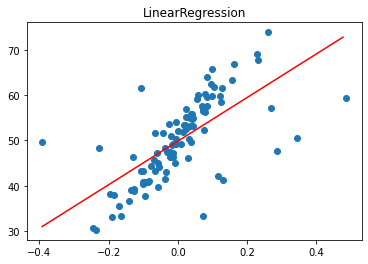
Before we start with mode details. let’s build up a simple linear regression so that we can compare each performance.
# linear regression with outliers
from random import random
from random import randint
from random import seed
from numpy import arange
from numpy import mean
from numpy import std
from numpy import absolute
from sklearn.datasets import make_regression
from sklearn.linear_model import LinearRegression
from sklearn.model_selection import cross_val_score
from sklearn.model_selection import RepeatedKFold
from matplotlib import pyplot

# prepare the dataset
def get_dataset():
 X, y = make_regression(n_samples=100, n_features=1, tail_strength=0.9, effective_rank=1, n_informative=1, noise=3, bias=50, random_state=1)
 # add some artificial outliers
 seed(1)
 for i in range(10):
  factor = randint(2, 4)
  if random() > 0.5:
   X[i] += factor * X.std()
  else:
   X[i] -= factor * X.std()
 return X, y

# evaluate a model
def evaluate_model(X, y, model):
 # define model evaluation method
 cv = RepeatedKFold(n_splits=10, n_repeats=3, random_state=1)
 # evaluate model
 scores = cross_val_score(model, X, y, scoring='neg_mean_absolute_error', cv=cv, n_jobs=-1)
 # force scores to be positive
 return absolute(scores)

# plot the dataset and the model's line of best fit
def plot_best_fit(X, y, model):
 # fut the model on all data
 model.fit(X, y)
 # plot the dataset
 pyplot.scatter(X, y)
 # plot the line of best fit
 xaxis = arange(X.min(), X.max(), 0.01)
 yaxis = model.predict(xaxis.reshape((len(xaxis), 1)))
 pyplot.plot(xaxis, yaxis, color='r')
 # show the plot
 pyplot.title(type(model).__name__)
 pyplot.show()

# load dataset
X, y = get_dataset()
# define the model
model = LinearRegression()
# evaluate model
results = evaluate_model(X, y, model)
print('Mean MAE: %.3f (%.3f)' % (mean(results), std(results)))
# plot the line of best fit
plot_best_fit(X, y, model)
Mean MAE: 5.260 (1.149)
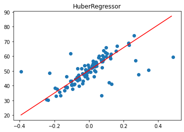
1. HuberRegressor
It is a type of robust regression that is aware of the possibility of outliers in a dataset and assigns them less weight than other examples in the dataset.
The “epsilon” argument controls what is considered an outlier, where smaller values consider more of the data outliers, and in turn, make the model more robust to outliers. The default is 1.35.
#huber regression with outliers
from random import random
from random import randint
from random import seed
from numpy import arange
from numpy import mean
from numpy import std
from numpy import absolute
from sklearn.datasets import make_regression
from sklearn.linear_model import HuberRegressor
from sklearn.model_selection import cross_val_score
from sklearn.model_selection import RepeatedKFold
from matplotlib import pyplot

# prepare the dataset
def get_dataset():
 X, y = make_regression(n_samples=100, n_features=1, tail_strength=0.9, effective_rank=1, n_informative=1, noise=3, bias=50, random_state=1)
 # add some artificial outliers
 seed(1)
 for i in range(10):
  factor = randint(2, 4)
  if random() > 0.5:
   X[i] += factor * X.std()
  else:
   X[i] -= factor * X.std()
 return X, y

# evaluate a model
def evaluate_model(X, y, model):
 # define model evaluation method
 cv = RepeatedKFold(n_splits=10, n_repeats=3, random_state=1)
 # evaluate model
 scores = cross_val_score(model, X, y, scoring='neg_mean_absolute_error', cv=cv, n_jobs=-1)
 # force scores to be positive
 return absolute(scores)

# plot the dataset and the model's line of best fit
def plot_best_fit(X, y, model):
 # fut the model on all data
 model.fit(X, y)
 # plot the dataset
 pyplot.scatter(X, y)
 # plot the line of best fit
 xaxis = arange(X.min(), X.max(), 0.01)
 yaxis = model.predict(xaxis.reshape((len(xaxis), 1)))
 pyplot.plot(xaxis, yaxis, color='r')
 # show the plot
 pyplot.title(type(model).__name__)
 pyplot.show()

# load dataset
X, y = get_dataset()
# define the model
model = HuberRegressor()
# evaluate model
results = evaluate_model(X, y, model)
print('Mean MAE: %.3f (%.3f)' % (mean(results), std(results)))
# plot the line of best fit
plot_best_fit(X, y, model)
Mean MAE: 4.435 (1.868)
Clearly, we can observe HuberRegressor outperforms better than our regular linear regression of MAE 5.260 (1.149)
2. RANSAC Regression
Random Sample Consensus, or RANSAC for short, is another robust regression algorithm. RANSAC tries to separate data into outliers and inliers and fits the model on the inliers.
# ransac regression with outliers
from random import random
from random import randint
from random import seed
from numpy import arange
from numpy import mean
from numpy import std
from numpy import absolute
from sklearn.datasets import make_regression
from sklearn.linear_model import RANSACRegressor
from sklearn.model_selection import cross_val_score
from sklearn.model_selection import RepeatedKFold
from matplotlib import pyplot

# prepare the dataset
def get_dataset():
 X, y = make_regression(n_samples=100, n_features=1, tail_strength=0.9, effective_rank=1, n_informative=1, noise=3, bias=50, random_state=1)
 # add some artificial outliers
 seed(1)
 for i in range(10):
  factor = randint(2, 4)
  if random() > 0.5:
   X[i] += factor * X.std()
  else:
   X[i] -= factor * X.std()
 return X, y

# evaluate a model
def evaluate_model(X, y, model):
 # define model evaluation method
 cv = RepeatedKFold(n_splits=10, n_repeats=3, random_state=1)
 # evaluate model
 scores = cross_val_score(model, X, y, scoring='neg_mean_absolute_error', cv=cv, n_jobs=-1)
 # force scores to be positive
 return absolute(scores)

# plot the dataset and the model's line of best fit
def plot_best_fit(X, y, model):
 # fut the model on all data
 model.fit(X, y)
 # plot the dataset
 pyplot.scatter(X, y)
 # plot the line of best fit
 xaxis = arange(X.min(), X.max(), 0.01)
 yaxis = model.predict(xaxis.reshape((len(xaxis), 1)))
 pyplot.plot(xaxis, yaxis, color='r')
 # show the plot
 pyplot.title(type(model).__name__)
 pyplot.show()

# load dataset
X, y = get_dataset()
# define the model
model = RANSACRegressor()
# evaluate model
results = evaluate_model(X, y, model)
print('Mean MAE: %.3f (%.3f)' % (mean(results), std(results)))
# plot the line of best fit
plot_best_fit(X, y, model)
Mean MAE: 4.476 (2.215)
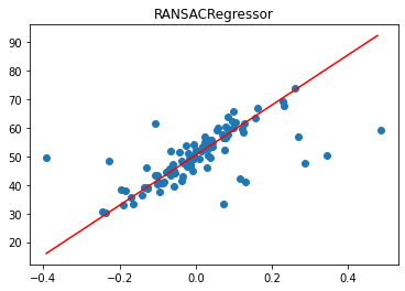
We can observe MAE of 4.54 outperforms Linear Regression.
3. Theil Sen Regression
involves fitting multiple regression models on subsets of the training data and combining the coefficients together in the end.
# theilsen regression with outliers
from random import random
from random import randint
from random import seed
from numpy import arange
from numpy import mean
from numpy import std
from numpy import absolute
from sklearn.datasets import make_regression
from sklearn.linear_model import TheilSenRegressor
from sklearn.model_selection import cross_val_score
from sklearn.model_selection import RepeatedKFold
from matplotlib import pyplot

# prepare the dataset
def get_dataset():
 X, y = make_regression(n_samples=100, n_features=1, tail_strength=0.9, effective_rank=1, n_informative=1, noise=3, bias=50, random_state=1)
 # add some artificial outliers
 seed(1)
 for i in range(10):
  factor = randint(2, 4)
  if random() > 0.5:
   X[i] += factor * X.std()
  else:
   X[i] -= factor * X.std()
 return X, y

# evaluate a model
def evaluate_model(X, y, model):
 # define model evaluation method
 cv = RepeatedKFold(n_splits=10, n_repeats=3, random_state=1)
 # evaluate model
 scores = cross_val_score(model, X, y, scoring='neg_mean_absolute_error', cv=cv, n_jobs=-1)
 # force scores to be positive
 return absolute(scores)

# plot the dataset and the model's line of best fit
def plot_best_fit(X, y, model):
 # fut the model on all data
 model.fit(X, y)
 # plot the dataset
 pyplot.scatter(X, y)
 # plot the line of best fit
 xaxis = arange(X.min(), X.max(), 0.01)
 yaxis = model.predict(xaxis.reshape((len(xaxis), 1)))
 pyplot.plot(xaxis, yaxis, color='r')
 # show the plot
 pyplot.title(type(model).__name__)
 pyplot.show()

# load dataset
X, y = get_dataset()
# define the model
model = TheilSenRegressor()
# evaluate model
results = evaluate_model(X, y, model)
print('Mean MAE: %.3f (%.3f)' % (mean(results), std(results)))
# plot the line of best fit
plot_best_fit(X, y, model)
Mean MAE: 4.371 (1.961)
Once again we can observe the TheilSenRegressor outperform all the above from linear regressor, huber and RANSAC regressor

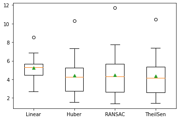
Let’s put all of them together ya! for a side-by-side comparison
# compare robust regression algorithms with outliers
from random import random
from random import randint
from random import seed
from numpy import mean
from numpy import std
from numpy import absolute
from sklearn.datasets import make_regression
from sklearn.model_selection import cross_val_score
from sklearn.model_selection import RepeatedKFold
from sklearn.linear_model import LinearRegression
from sklearn.linear_model import HuberRegressor
from sklearn.linear_model import RANSACRegressor
from sklearn.linear_model import TheilSenRegressor
from matplotlib import pyplot

# prepare the dataset
def get_dataset():
 X, y = make_regression(n_samples=100, n_features=1, tail_strength=0.9, effective_rank=1, n_informative=1, noise=3, bias=50, random_state=1)
 # add some artificial outliers
 seed(1)
 for i in range(10):
  factor = randint(2, 4)
  if random() > 0.5:
   X[i] += factor * X.std()
  else:
   X[i] -= factor * X.std()
 return X, y

# dictionary of model names and model objects
def get_models():
 models = dict()
 models['Linear'] = LinearRegression()
 models['Huber'] = HuberRegressor()
 models['RANSAC'] = RANSACRegressor()
 models['TheilSen'] = TheilSenRegressor()
 return models

# evaluate a model
def evalute_model(X, y, model, name):
 # define model evaluation method
 cv = RepeatedKFold(n_splits=10, n_repeats=3, random_state=1)
 # evaluate model
 scores = cross_val_score(model, X, y, scoring='neg_mean_absolute_error', cv=cv, n_jobs=-1)
 # force scores to be positive
 scores = absolute(scores)
 return scores

# load the dataset
X, y = get_dataset()
# retrieve models
models = get_models()
results = dict()
for name, model in models.items():
 # evaluate the model
 results[name] = evalute_model(X, y, model, name)
 # summarize progress
 print('>%s %.3f (%.3f)' % (name, mean(results[name]), std(results[name])))
# plot model performance for comparison
pyplot.boxplot(results.values(), labels=results.keys(), showmeans=True)
pyplot.show()
>Linear 5.260 (1.149)
>Huber 4.435 (1.868)
>RANSAC 4.492 (2.272)
>TheilSen 4.371 (1.961)
That’s it.
It’s great to know all these new advanced techniques. Likewise, I will try to bring the best of machine learning from across as much as possible.
Thanks again, for your time, if you enjoyed this short article there are tons of topics in advanced analytics, data science, and machine learning available in my medium repo. https://medium.com/@bobrupakroy
Some of my alternative internet presences Facebook, Instagram, Udemy, Blogger, Issuu, Slideshare, Scribd and more.
Also available on Quora @ https://www.quora.com/profile/Rupak-Bob-Roy
Let me know if you need anything. Talk Soon.


Comments
Post a Comment