Yes! now convert all your sklearn models to time series model
Hello there, today we will discuss how to convert our regular sklearn machine learning models into time series models.
Before we get started let's recap how the time series works.
There are tons of articles available over the net even from my previous time series articles. Now if you remember the time series internally works as autoregressor and also ifyou remember the formula of the regressor
y = mx+ c, where m = beta coefficients, x = x1, c = intercept
And if you remember how time series work, using Autoregressor
i.e. X(t+1) = c +m1*(t-1) + m2*(t-2)…… so on and so forth.
Autoregressor itself is multivariate in the sense it computes t+1 with its lag version of itself and this is how time series works!
Now offcourse there are a few other components of time series like identifying the trend, and seasonality which gets identified and removed while moving ahead to the autoregressor component.
There are again various ways to remove the seasonality one of the common well know methods is Differencing if you wish to apply Arima
In this article, we will explore a number of ways to change the default autoregressor into our favorite regressor of all time like XGboost.
Let’s get started.
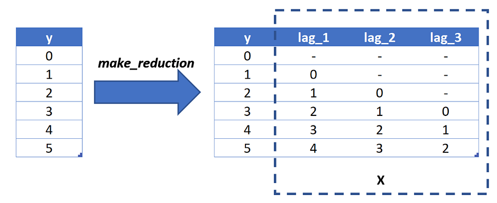
The first thing we need to take care of is formating the target attribute ‘y’ into a supervised learning dataset format.
make_reduction
The more lag version we create the more we can forecast based upon, that doesn't mean you can forecast X100times, offcourse the further you forecast the confidence level of accuracy will be lesser. if not then it's a GOD MODE :)
To order to perform such a conversation we can create a custom function or we can now simply use ‘make_reduction’ from sktime package.
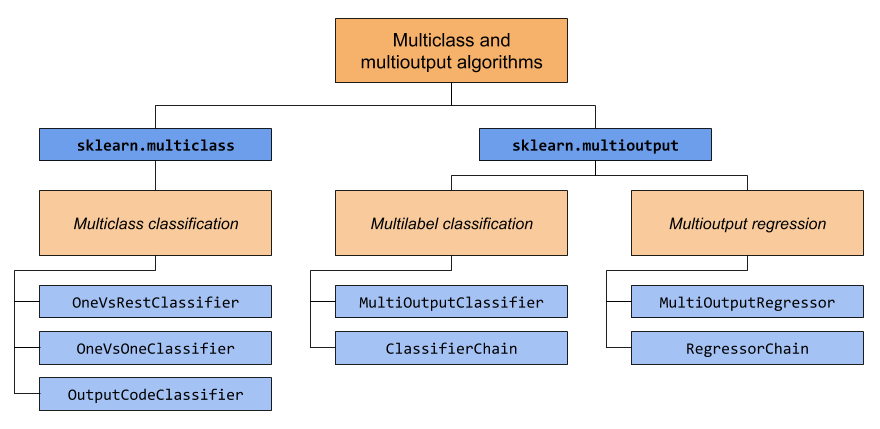
Strategy =Direct, we will see below we will create 26-step forecasting. therefore strategy = “Direct” will create a separate model for each period like 26 models for 26-step forecasting each model making its single-step prediction.
Strategy = Recursive, here we will use the previous time step’s output for the next step’s input recursively for N number of forecasts. Thus we will fit the one-step ahead model.
Strategy = Multiple outputs, here one model will be used to predict the entire time series in a single forecast.
We can also achieve the above step with the Regressor Chain method which will learn in another article.
Alternative to skltime
Window_length: is the same the window size.
Here are some quick definitions of Window size i was able to gather. What is a good window size for moving average? If we simply look at a plot of our data we can already discover a weekly pattern. Hence, for our data a moving average of window size 7 seems suitable for capturing the trend cycle.
Usually windowing is done to smooth your time series and thus reduce noise and let you see trends more clearly in your data. A larger window gives more smoothing but obscures high frequency features. If your interest is in predicting beyond the end of the time series, there is no advantage to windowing other than perhaps letting you choose a good fitting function. Just do a least-squares regression fit to the raw data and extrapolate. Beware, accurate prediction is difficult, especially of the future.
In time series problem, this duration is called window length or time lags. It represents the number of time steps in the time series to be inserted as input for the predictive model.
sktime’s temporal_train_test_split function does not shuffle the data. Therefore it is suitable for forecasting.
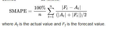
def smape(A, F):
return 100/len(A) * np.sum(2 * np.abs(F - A) / (np.abs(A) + np.abs(F)))
#Method 2
def smape(A, F):
tmp = 2 * np.abs(F - A) / (np.abs(A) + np.abs(F))
len_ = np.count_nonzero(~np.isnan(tmp))
if len_ == 0 and np.nansum(tmp) == 0: # Deals with a special case
return 100
return 100 / len_ * np.nansum(tmp)
smape(y_test, y_pred)
#8.661467738190655
Above quick a function to calculate the SMAPE, smape also have advantages and disadvantages which we discussed in my previous article, you can also use the MSE, or MAE. no harm.
#Now we will apply XGBOOST
from sktime.forecasting.compose import make_reduction
import xgboost
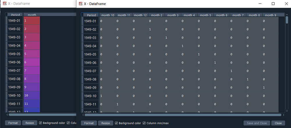
# Create an exogenous dataframe indicating the month
X = pd.DataFrame({'month': y.index.month}, index=y.index)
X = pd.get_dummies(X.astype(str), drop_first=True)
X_train, X_test = temporal_train_test_split(X, test_size=36)
regressor = xgboost.XGBRegressor(objective='reg:squarederror', random_state=42)
forecaster = make_reduction(regressor, window_length=12, strategy="recursive")
# Fit and predict
forecaster.fit(y=y_train, X=X_train)
y_pred = forecaster.predict(fh=fh, X=X_test)
# Evaluate
mean_absolute_percentage_error(y_test, y_pred)
#0.10052889328976747
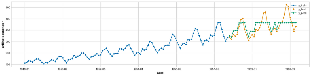
# Plot predictions with training and test data
plot_series(y_train, y_test, y_pred, labels=["y_train", "y_test", "y_pred"], x_label='Date', y_label='ariline passenger');
# Create an exogenous dataframe indicating the month X = pd.DataFrame({‘month’: y.index.month}, index=y.index) X = pd.get_dummies(X.astype(str), drop_first=True) XGBOOST Time Series Well well well, i would say it's a reasonably good fit. neither over nor underfit the predictions. the Xgboost’s default parameters. That’s it! done….Congratulations….mate now you can use any sklearn models like random forest, extratreesregressor, linear regression etc.Moving ahead we will continue to explore “How to perform time series classification.”
from sktime.classification.all import *
from sklearn.model_selection import train_test_split
from sklearn.metrics import accuracy_score
X, y = load_arrow_head(return_X_y=True)
X_train, X_test, y_train, y_test = train_test_split(X, y)
classifier = TimeSeriesForestClassifier()
classifier.fit(X_train, y_train)
y_pred = classifier.predict(X_test)
accuracy_score(y_test, y_pred)
#0.8867924528301887
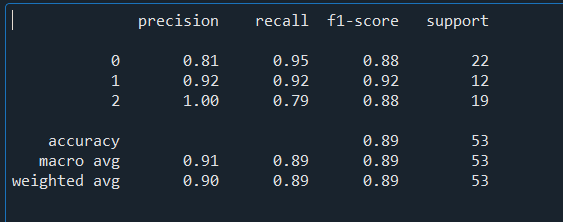
from sklearn.metrics import confusion_matrix,classification_report
cm = confusion_matrix(y_test, y_pred)
cm
report = classification_report(y_test,y_pred,output_dict=False)
A single time series variable and a corresponding label for multiple instances. The aim is to find a suitable classifier model that can be used to learn the relationship between time-series data and label and predict likewise the new series’s label.
import matplotlib.pyplot as plt import numpy as np from sklearn.metrics import accuracy_score from sklearn.model_selection import train_test_split from sklearn.pipeline import Pipeline from sklearn.tree import DecisionTreeClassifier #from sktime.classification.compose import TimeSeriesForestClassifier from sktime.classification.all import * from sktime.datasets import load_arrow_head from sktime.utils.slope_and_trend import _slope
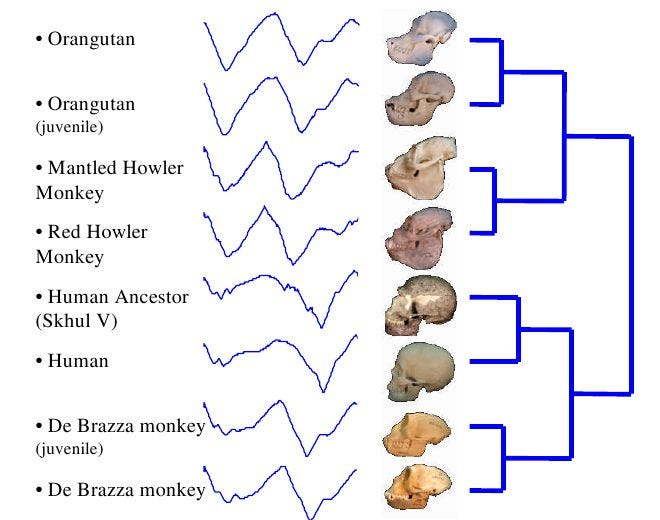
The arrowhead dataset is a time-series dataset containing outlines of the images of arrowheads. In anthropology, the classification of projectile points is an important topic. The classes are categorized based on shape distinctions eg. — the presence and location of a notch in the arrow.
The shapes of the projectile points are to be converted into sequences using the angle-based method.
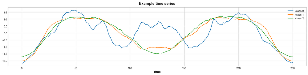
fig, ax = plt.subplots(1, figsize=plt.figaspect(0.25)) for label in labels: X_train.loc[y_train == label, "dim_0"].iloc[0].plot(ax=ax, label=f"class {label}") plt.legend() ax.set(title="Example time series", xlabel="Time");
Image to Time Series Plot
TIME SERIES FOREST Time series forest is a modification of the random forest algorithm to the time series setting:
Splitting the series into multiple random intervals, Extracting features (mean, standard deviation and slope) from each interval, Training a decision tree on the extracted features, Ensembling steps 1–3.
from sktime.transformations.panel.summarize import RandomIntervalFeatureExtractor
Done. That's it… i hope you enjoyed the AAAdditional* input Univariate and TimeSeriesForest………..
i hope you enjoyed likewise, i will try to bring as much as possible new contents across the data science realm and i hope the package will be useful at some point in your work. Because I believe machine learning is not replacing us, it’s about replacing the same iterative work that consumes time and much effort. So people should come to work to create innovations rather than be occupied in the same repetitive boring tasks.
Thanks again, for your time, if you enjoyed this short article there are tons of topics in advanced analytics, data science, and machine learning available in my medium repo. https://medium.com/@bobrupakroy
Some of my alternative internet presencesFacebook, Instagram, Udemy, Blogger, Issuu, Slideshare, Scribd and more.


Comments
Post a Comment