Bias-Variance Decomposition. Implementing quadratic risk function to sklearn classifiers, regressors and keras/tensorflow

 

Bias-Variance Decomposition. 

Implementing quadratic risk function to sklearn classifiers, regressors and keras/tensorflow

Hi there, whatsup? things are going great? hope so.

just like old times today we will discuss something new ya!.

So what is New?

— — — — — — Bias Variance Trade-off, well you might be thinking its an old stuff but have you applied that anytime in your real-life ml use case?

90% no. we just read the theory that's it. That not gonna work! Let’s learn this cool feature that will set us ahead of others :)

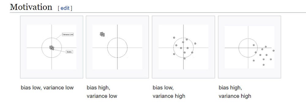
A small recap: Bias-Variance trade-off

Wiki: In statistics and machine learning, the bias–variance tradeoff is the property of a model that the variance of the parameter estimated across samples can be reduced by increasing the bias in the estimated parameters. The bias–variance dilemma or bias–variance problem is the conflict in trying to simultaneously minimize these two sources of error that prevent supervised learning algorithms from generalizing beyond their training set:[1][2]

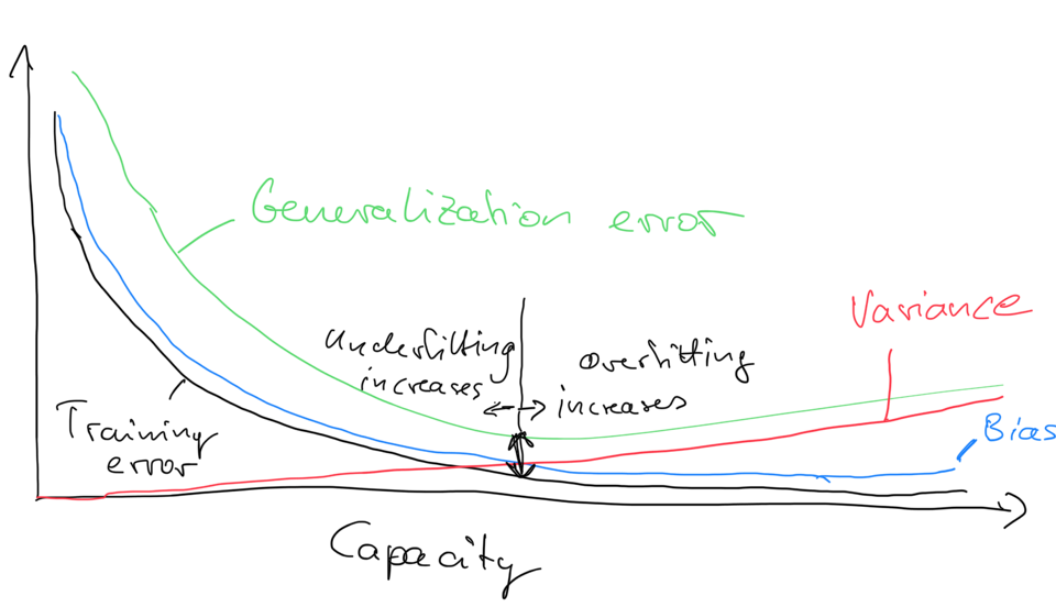
• The bias error is an error from erroneous assumptions in the learning algorithm. High bias can cause an algorithm to miss the relevant relations between features and target outputs (underfitting).
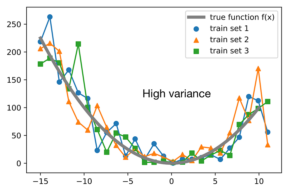
• The variance is an error from sensitivity to small fluctuations in the training set. High variance may result from an algorithm modeling the random noise in the training data (overfitting).

We need Low Bias Low Variance | image:wiki

To use the more formal terms for bias and variance, assume we have a point estimator θ^(theta hat)of some parameter or function θ. Then, the bias is commonly defined as the difference between the expected value of the estimator and the parameter that we want to estimate:

Bias=E[θ^]−θ.Bias=E[θ^]−θ.

If the bias is larger than zero, we also say that the estimator is positively biased, if the bias is smaller than zero, the estimator is negatively biased, and if the bias is exactly zero, the estimator is unbiased. Similarly, we define the variance as the difference between the expected value of the squared estimator minus the squared expectation of the estimator:

Var(θ^)=E[θ²]−(E[θ^])2.Var(θ^)=E[θ²]−(E[θ^])2.

Note that in the context of this lecture, it will be more convenient to write the variance in its alternative form:

Var(θ^)=E[(E[θ^]−θ^)2].

Heard of MSE? off-course you had! what a silly question

MSE is a risk function, corresponding to the expected value of the squared error loss. The fact that MSE is almost always strictly positive (and not zero) is because of randomness or because the estimator does not account for information that could produce a more accurate estimate.

MSE may refer to the empirical risk (the average loss on an observed data set), as an estimate of the true MSE (the true risk: the average loss on the actual population distribution)

The MSE is the second moment (about the origin) of the error, and thus incorporates both the variance of the estimator (how widely spread the estimates are from one data sample to another) and its bias (how far off the average estimated value is from the true value)

For an unbiased estimator, the MSE is the variance of the estimator. Like the variance, MSE has the same units of measurement as the square of the quantity being estimated.

for more detailed info: https://en.wikipedia.org/wiki/Mean_squared_error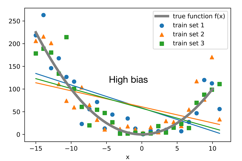

high bias | image: mlxtend

high variance | image: mlxtend

How high variance related to overfitting, and how large bias relates to underfitting | image: mlxtend

We gonna skip the theory there are tons of information, and articles on this. We are more interested to see how to apply in our Machine Learning Models.

Simple words: Quadratic Risk = Variance + Bias²

Let’s get started!

Bias-Variance Decomposition of the 0–1 Loss

Note that decomposing the 0–1 loss into bias and variance components is not as straightforward as for the squared error loss. To quote Pedro Domingos, a well-known machine learning researcher and professor at University of Washington:

“several authors have proposed bias-variance decompositions related to zero-one loss (Kong & Dietterich, 1995; Breiman, 1996b; Kohavi & Wolpert, 1996; Tibshirani, 1996; Friedman, 1997). However, each of these decompositions has significant shortcomings.”.

Recall that the 0–1 loss, LL, is 0 if a class label is predicted correctly, and one otherwise.

Example 1 — Bias Variance Decomposition of a Decision Tree Classifier

from mlxtend.evaluate import bias_variance_decomp
from sklearn.tree import DecisionTreeClassifier
from mlxtend.data import iris_data
from sklearn.model_selection import train_test_split

X, y = iris_data()
X_train, X_test, y_train, y_test = train_test_split(X, y,
                                                    test_size=0.3,
                                                    random_state=123,
                                                    shuffle=True,
                                                    stratify=y)

tree = DecisionTreeClassifier(random_state=123)

avg_expected_loss, avg_bias, avg_var = bias_variance_decomp(
        tree, X_train, y_train, X_test, y_test, 
        loss='0-1_loss',
        random_seed=123)

print('Average expected loss: %.3f' % avg_expected_loss)
print('Average bias: %.3f' % avg_bias)
print('Average variance: %.3f' % avg_var)

For comparison, the bias-variance decomposition of a bagging classifier, which should intuitively have a lower variance compared than a single decision tree:

from sklearn.ensemble import BaggingClassifier

tree = DecisionTreeClassifier(random_state=123)
bag = BaggingClassifier(base_estimator=tree,
                        n_estimators=100,
                        random_state=123)

avg_expected_loss, avg_bias, avg_var = bias_variance_decomp(
        bag, X_train, y_train, X_test, y_test, 
        loss='0-1_loss',
        random_seed=123)

print('Average expected loss: %.3f' % avg_expected_loss)
print('Average bias: %.3f' % avg_bias)
print('Average variance: %.3f' % avg_var)

Example 2 — Bias Variance Decomposition of a Decision Tree Regressor

from mlxtend.evaluate import bias_variance_decomp
from sklearn.tree import DecisionTreeRegressor
from mlxtend.data import boston_housing_data
from sklearn.model_selection import train_test_split

X, y = boston_housing_data()
X_train, X_test, y_train, y_test = train_test_split(X, y,
                                                    test_size=0.3,
                                                    random_state=123,
                                                    shuffle=True)

tree = DecisionTreeRegressor(random_state=123)

avg_expected_loss, avg_bias, avg_var = bias_variance_decomp(
        tree, X_train, y_train, X_test, y_test, 
        loss='mse',
        random_seed=123)

print('Average expected loss: %.3f' % avg_expected_loss)
print('Average bias: %.3f' % avg_bias)
print('Average variance: %.3f' % avg_var)

For comparison, the bias-variance decomposition of a bagging regressor is shown below, which should intuitively have a lower variance than a single decision tree:

from sklearn.ensemble import BaggingRegressor

tree = DecisionTreeRegressor(random_state=123)
bag = BaggingRegressor(base_estimator=tree,
                       n_estimators=100,
                       random_state=123)

avg_expected_loss, avg_bias, avg_var = bias_variance_decomp(
        bag, X_train, y_train, X_test, y_test, 
        loss='mse',
        random_seed=123)

print('Average expected loss: %.3f' % avg_expected_loss)
print('Average bias: %.3f' % avg_bias)
print('Average variance: %.3f' % avg_var)

Example 3 — TensorFlow/Keras Support

Since mlxtend v0.18.0, the bias_variance_decomp now supports Keras models. Note that the original model is reset in each round (before refitting it to the bootstrap samples).

from mlxtend.evaluate import bias_variance_decomp
from mlxtend.data import boston_housing_data
from sklearn.model_selection import train_test_split
from sklearn.metrics import mean_squared_error
import tensorflow as tf
import numpy as np

np.random.seed(1)
tf.random.set_seed(1)

X, y = boston_housing_data()
X_train, X_test, y_train, y_test = train_test_split(X, y,
                                                    test_size=0.3,
                                                    random_state=123,
                                                    shuffle=True)

model = tf.keras.Sequential([
    tf.keras.layers.Dense(32, activation=tf.nn.relu),
    tf.keras.layers.Dense(1)
  ])

optimizer = tf.keras.optimizers.Adam()
model.compile(loss='mean_squared_error', optimizer=optimizer)

model.fit(X_train, y_train, epochs=100, verbose=0)

mean_squared_error(model.predict(X_test), y_test)

32.69300595184836

Note that it is highly recommended to use the same number of training epochs that you would use on the original training set to ensure convergence:

np.random.seed(1)
tf.random.set_seed(1)

avg_expected_loss, avg_bias, avg_var = bias_variance_decomp(
        model, X_train, y_train, X_test, y_test, 
        loss='mse',
        num_rounds=100,
        random_seed=123,
        epochs=200, # fit_param
        verbose=0) # fit_param

print('Average expected loss: %.3f' % avg_expected_loss)
print('Average bias: %.3f' % avg_bias)
print('Average variance: %.3f' % avg_var)

Repo:http://rasbt.github.io/mlxtend/user_guide/evaluate/bias_variance_decomp/

Well, that's it!

Thanks to mlxtend team and to me also ya? for bringing up this to you?

I hope you find this article useful for your machine learning and statistical use cases. Likewise, i will try to bring new ways across with the motto “curiosity leads to innovation” :)

Check out the kaggle implementation: https://www.kaggle.com/code/rupakroy/bias-variance-decomposition

Thanks again, for your time, if you enjoyed this short article there are tons of topics in advanced analytics, data science, and machine learning available in my medium repo. https://medium.com/@bobrupakroy

Some of my alternative internet presences are Facebook, Instagram, Udemy, Blogger, Issuu, Slideshare, Scribd and more.

Also available on Quora @ https://www.quora.com/profile/Rupak-Bob-Roy

Let me know if you need anything. Talk Soon.