Calibration for Actual Probabilities using isotonic, logistic regression and calibratedclassifierCV

Hi everyone, hope you are doing awesome.
Today we have something very surprising and interesting to know about.
It's called Calibration.
We are aware that most machine learning models for classification result in between 0 and 1which again can be interpreted into probabilities by calling predict_proba().
But there is a catch when we do it in iterations. Let’s say we have used a random forest, which is an ensemble method having the number of decision trees. The random forest’s prediction is done by averaging individual decision tree results, Correct?
Now let's say a model predicted a probability of zero for some sample data. And for sure the other individual ensembled decision trees results will predict a slightly higher value. Taking the average will push the random forest’s overall prediction away from Zero. Makes Sense?
That's why we need calibration of our probability scores. The idea of probability calibration is to build a second model (called calibrator) that is able to correct them into actual probabilities.
Calibration consists of a function that transforms a -1 dimensional vector (uncalibrated probabilities) into another 1-dimensions vector (of calibrated probabilities)
Let’s take another example. if your model outputs a prediction of heart failure in the next months, the doctors for sure will start acting on the people whose risk is above 0.5+ probability score, now if your model prediction is not calibrated, the model outputs may mislead anyone taking action based on its immediate model outputs. A calibrated model with a score 0.8 probability will actually mean that the instance has an 80% chance of being True.
The easiest way to assess the calibration of your model is through a plot called calibration curve (a.k.a. “reliability diagram”).
“The idea is to divide the observations into bins of probability.
Thus, observations that belong to the same bin share a similar probability.
At this point, for each bin, the calibration curve compares the predicted mean (i.e. mean of the predicted probability) with the theoretical mean (i.e. mean of the observed target variable).’’
The calibration curve with an S-shaped pattern is often the case for many classification models and the consequence is usually over-forecasting low probabilities and under forecasting high probabilities.
There are 3 methods used as calibrators:
- Logistic Regression. Logistic regression is a rate beast that actually produces calibrated probabilities, the reason behind that is it optimizes for log-odds, which makes probabilities actually present in the model’s cost function. It is also known as Platt-scaling.
- Isotonic Regression. It’s a non-parametric model that fits a piecewise function to the outputs.
- CalibratedClassifierCV. Probability classifier with isotonic regression or logistic regression from sklearn
calibrating the model does not guarantee an improvement in the existing model class accuracy, metrics like accuracy, precision, or recall also play an important role.
The most common types of miscalibration are:
l. Systematic overestimation. Compared to the true distribution, the distribution of predicted probabilities is pushed towards the right. This is common when you train a model on an unbalanced dataset with very few positives.
2. Systematic underestimation. Compared to the true distribution, the distribution of predicted probabilities is pushed leftward.
3. Center of the distribution is too heavy. This happens when “algorithms such as support vector machines and boosted trees tend to push predicted probabilities away from 0 and 1” (quote from «Predicting good probabilities with supervised learning»).
4. Tails of the distribution are too heavy. For instance, “Other methods such as naive Bayes have the opposite bias and tend to push predictions closer to 0 and 1” (quote from «Predicting good probabilities with supervised learning»).
Other use cases:
Ensembling: when we want to combine many probability models having uncalibrated predictions makes a difference.
from sklearn.datasets import make_classification
X, y = make_classification(
    n_samples = 15000,
    n_features = 50,
    n_informative = 30,
    n_redundant = 20,
    weights = [.9, .1],
    random_state = 0
)
X_train, X_valid, X_test = X[:5000], X[5000:10000], X[10000:]
y_train, y_valid, y_test = y[:5000], y[5000:10000], y[10000:]
from sklearn.ensemble import RandomForestClassifier
forest = RandomForestClassifier().fit(X_train, y_train)
proba_valid = forest.predict_proba(X_valid)[:, 1]
#using sklearn
from sklearn import calibration
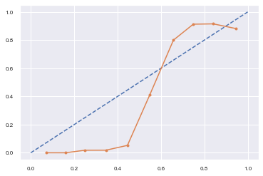
#Random forest
y_means, proba_means =calibration.calibration_curve(y_valid,proba_valid, normalize=False, n_bins=5,
strategy='uniform')
import matplotlib.pyplot as plt
plt.plot([0, 1], [0, 1], linestyle = '--', label = 'Perfect calibration')
plt.plot(proba_means, y_means)
plt.show()
1. random forest
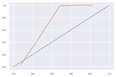
2. random forest + isotonic regression
3. random forest + logistic regression
#Isotonic regression
from sklearn.isotonic import IsotonicRegression
iso_reg = IsotonicRegression(y_min = 0, y_max = 1, out_of_bounds = 'clip').fit(proba_valid, y_valid)
proba_test_forest_isoreg = iso_reg.predict(forest.predict_proba(X_test)[:, 1])
#Logistic regression:
from sklearn.linear_model import LogisticRegression
log_reg = LogisticRegression().fit(proba_valid.reshape(-1, 1), y_valid)
proba_test_forest_logreg = log_reg.predict_proba(forest.predict_proba(X_test)[:, 1].reshape(-1, 1))[:, 1]
Metrics to assess which one is better calibrated. Expected Calibration Error gives how far away is our predicted probability from the true actual probability
# Freedman-Diaconis rule
def expected_calibration_error(y, proba, bins = 'fd'):
  import numpy as np
  bin_count, bin_edges = np.histogram(proba, bins = bins)
  n_bins = len(bin_count)
  bin_edges[0] -= 1e-8 # because left edge is not included
  bin_id = np.digitize(proba, bin_edges, right = True) - 1
  bin_ysum = np.bincount(bin_id, weights = y, minlength = n_bins)
  bin_probasum = np.bincount(bin_id, weights = proba, minlength = n_bins)
  bin_ymean = np.divide(bin_ysum, bin_count, out = np.zeros(n_bins), where = bin_count > 0)
  bin_probamean = np.divide(bin_probasum, bin_count, out = np.zeros(n_bins), where = bin_count > 0)
  ece = np.abs((bin_probamean - bin_ymean) * bin_count).sum() / len(proba)
  return ece
#random forest
expected_calibration_error(y_valid, proba_valid)
#random forest + isotonic regression
expected_calibration_error(y_valid, proba_test_forest_isoreg)
#random forest + logistic regression
expected_calibration_error(y_valid, proba_test_forest_logreg)
Random Forest: 0.07475200000000007
Random Forest + Isotonic Regression: 0.138570621223946
Random Forest + logistic regression: 0.11915893242619713
Now its try with CalibratedClassifierCV
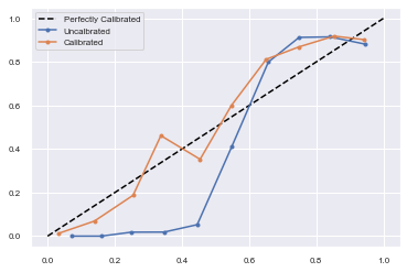
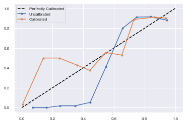
# SVM reliability diagrams with uncalibrated and calibrated probabilities
from sklearn.datasets import make_classification
from sklearn.svm import SVC
from sklearn.calibration import CalibratedClassifierCV
from sklearn.model_selection import train_test_split
from sklearn.calibration import calibration_curve
from matplotlib import pyplot

# predict uncalibrated probabilities
def uncalibrated(trainX, testX, trainy):
 # fit a model
 model = SVC()
 model.fit(trainX, trainy)
 # predict probabilities
 return model.decision_function(testX)

# predict calibrated probabilities
def calibrated(trainX, testX, trainy):
 # define model
 model = SVC()
 # define and fit calibration model
 calibrated = CalibratedClassifierCV(model, method='sigmoid', cv=5)
#calibrated = CalibratedClassifierCV(model, method='isotonic', cv=5)
 calibrated.fit(trainX, trainy)
 # predict probabilities
 return calibrated.predict_proba(testX)[:, 1]

#create binary 2class dataset
X, y = make_classification(n_samples=1000, n_classes=2, weights=[1,1], random_state=1)
# split into train/test sets
trainX, testX, trainy, testy = train_test_split(X, y, test_size=0.5, random_state=2)
# uncalibrated predictions
yhat_uncalibrated = uncalibrated(trainX, testX, trainy)
# calibrated predictions
yhat_calibrated = calibrated(trainX, testX, trainy)
# reliability diagrams
fop_uncalibrated, mpv_uncalibrated = calibration_curve(testy, yhat_uncalibrated, n_bins=10, normalize=True)
fop_calibrated, mpv_calibrated = calibration_curve(testy, yhat_calibrated, n_bins=10)
# plot perfectly calibrated
pyplot.plot([0, 1], [0, 1], linestyle='--', color='black')
# plot model reliabilities
pyplot.plot(mpv_uncalibrated, fop_uncalibrated, marker='.')
pyplot.plot(mpv_calibrated, fop_calibrated, marker='.')
pyplot.legend(["Perfectly Calibrated","Uncalbrated","Calibrated"])
pyplot.show()
THE END — — — — — — —
BUT if you find this article useful…. do browse my other ensemble techniques like Bagging Classifier, Voting Classifier, Stacking, and more I guarantee you will like them too. See you soon with another interesting topic.
The outlier detection for feature spaces with low dimensionalitybobrupakroy.medium.com
Some of my alternative internet presences are Facebook, Instagram, Udemy, Blogger, Issuu, and more.
Also available on Quora @ https://www.quora.com/profile/Rupak-Bob-Roy
Have a good day. Talk Soon.


Comments
Post a Comment