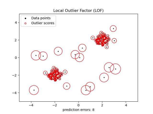
Local Outlier Factor (LOF). The outlier detection for feature spaces with low dimensionality

Apart from our traditional quantile-based outlier treatment I’m gonna show you another quick way to identify outliers when you have low features.

Local Outlier Factor (LOF)

A simple approach to identify outliers when we have features spaces with low dimensionality that works well with low features. Local Outlier Factor technique harness the working of nearest neighbors for outlier detection. This we will find the algorithm from sklearn.neighbors.

Let’s get started…..

import numpy as np 
import pandas as pd
from sklearn.model_selection import train_test_split
from sklearn.metrics import mean_absolute_error

df = pd.read_csv("housing.csv")
data = df.values

#define the X and y
X, y = data[:, :-1], data[:, -1]# split into train and test sets
X_train, X_test, y_train, y_test = train_test_split(X, y, test_size=0.33, random_state=1)

Once we are done with loading the dataset and split, we will apply LOF

from sklearn.neighbors import LocalOutlierFactor

# identify outliers in the training dataset
lof = LocalOutlierFactor()
yhat = lof.fit_predict(X_train)

# select all rows that are not outliers
mask = yhat != -1
X_train, y_train = X_train[mask, :], y_train[mask]

#Else impute the outliers with nan then replace with mean or median
#mask = yhat ==-1
#Impute with nan
#-----replace with mean or median----

A few more parameters of LocalOutlierFactor includes

LocalOutlierFactor(*, self, n_neighbors=20, algorithm=’auto’, leaf_size=30, metric=’minkowski’, p=2, metric_params=None, contamination=”auto”, novelty=False, n_jobs=None)

Now we can carry forward our cleaned dataset for any modeling tasks.

from sklearn.model_selection import KFold, cross_val_score
kfold =KFold(n_splits=3)
#no. of base classifiers
num_trees = 500

from sklearn.tree import DecisionTreeRegressor
from sklearn.ensemble import BaggingRegressor

#bagging classifier
model_regressor = BaggingRegressor(base_estimator = DecisionTreeRegressor(),n_estimators=num_trees,random_state=3)
results1 =cross_val_score(model_regressor,X_train,y_train,cv = kfold)
results1.mean()

model_regressor.fit(X_train,y_train)
model_regressor.predict(X_test)

# evaluate the model
yhat = model_regressor.predict(X_test)
# evaluate predictions
mae = mean_absolute_error(y_test, yhat)
print('MAE: %.3f' % mae)

Done…!

Now with our Traditional Quantile Based Outlier Detection Approach, we have to perform one column at a time.

import seaborn as sns

sns.boxplot(col_name)#to visualize the outliers

q1 = df['col_name'].quantile(0.25) #first quartile value
q3 = df['col_name'].quantile(0.75) # third quartile value

iqr = q3-q1 #Interquartile range

low  = q1-1.5*iqr #acceptable range
high = q3+1.5*iqr #acceptable range

#capping approach 
#to replace the extreme values with the acceptable range
df.loc[df["col_name"] <low, "col_name"] = low
df.loc[df["col_name"] >high, "col_name"] = high

Congrats on our previous article we have performed 4 different types of Anomaly / Outlier Detection from the traditional approach to the advanced robust approach.

If you like to know more about advanced topics like clustering follow my other article A-Z clustering

Some of my alternative internet presences are Facebook, Instagram, Udemy, Blogger, Issuu, and more.

Also available on Quora @ https://www.quora.com/profile/Rupak-Bob-Roy

Have a good day.