Borderline KNN| SVM and ADAYSN SMOTE ~ Complete walkthrough the various advanced variants of SMOTE

As promised in our previous article today we will look into the variants of SMOTE.
- Borderline SMOTE KNN
- Borderline SMOTE SVM
- Adaptive Synthetic Sampling (ADASYN)
My previous article link https://bob-rupak-roy.medium.com/synthetic-minority-oversampling-technique-smote-5bef8e3577d6
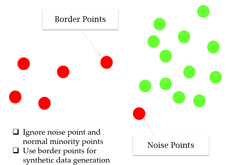
Borderline SMOTE
Instead of generating new synthetic data for the minority class blindly, the Borderline-SMOTE method will create synthetic data along the decision boundary between the two classes.
Let me explain you with the help of an example
#Borderline-SMOTE KNN
from collections import Counter
from sklearn.datasets import make_classification
from imblearn.over_sampling import BorderlineSMOTE
from matplotlib import pyplot
from numpy import where
#Create Imbalanced Class dataset
X, y = make_classification(n_samples=10000, n_features=2, n_redundant=0, n_clusters_per_class=1, weights=[0.99], flip_y=0, random_state=1)
counter = Counter(y)
Counter({0: 9900, 1: 100}) #Ratio before resampling
#Apply Borderline-SMOTE
oversample = BorderlineSMOTE()
X, y = oversample.fit_resample(X, y)
counter = Counter(y)
Counter({0: 9900, 1: 9900}) #Ratio after resampling
Let’s visualize the data and see what we got.
for label, _ in counter.items():
 row_ix = where(y == label)[0]
 pyplot.scatter(X[row_ix, 0], X[row_ix, 1], label=str(label))
pyplot.legend()
pyplot.show()
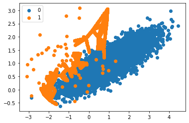
We can observe that the observation/data points that are far from the decision boundary are not oversampled.
Let’s see what is the difference we get with Borderline SMOTE SVM
2. Borderline SMOTE SVM
#Borderline-SMOTE SVM
from collections import Counter
from sklearn.datasets import make_classification
from imblearn.over_sampling import SVMSMOTE
from matplotlib import pyplot
from numpy import where
#Create Imbalanced Class dataset
X, y = make_classification(n_samples=10000, n_features=2, n_redundant=0,
 n_clusters_per_class=1, weights=[0.99], flip_y=0, random_state=1)
counter = Counter(y)
Counter({0: 9900, 1: 100}) #Ratio before resampling
#Apply the SVMSMOTE
oversample = SVMSMOTE()
X, y = oversample.fit_resample(X, y)
counter = Counter(y)
Counter({0: 9900, 1: 9900}) #Ratio after resampling
Visualizing the output
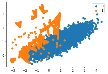
We can observe more synthesized data generated towards the top left of the plot instead of class overlap
Next, we have another approach that involves generating synthetic data inversely proportional to the density of the data in the minority class.
3.) Adaptive Synthetic Sampling (ADASYN)
It tries to generate more synthetic data in regions of the feature space/areas where the density of minority examples is low and fewer or none where the density is high.
The idea behind ADASYN is to use density distribution as a main criteria to generate synthetic samples for each minority class.
#ADASYN
from collections import Counter
from sklearn.datasets import make_classification
from imblearn.over_sampling import ADASYN
from matplotlib import pyplot
from numpy import where
#Create Imbalanced Class dataset
X, y = make_classification(n_samples=10000, n_features=2, n_redundant=0,
 n_clusters_per_class=1, weights=[0.99], flip_y=0, random_state=1)
counter = Counter(y)
Counter({0: 9900, 1: 100}) #Ratio before resampling
#Apply the ADASYN
oversample = ADASYN()
X, y = oversample.fit_resample(X, y)
counter = Counter(y)
Counter({0: 9900, 1: 9899}) #Ratio after resampling
for label, _ in counter.items():
 row_ix = where(y == label)[0]
 pyplot.scatter(X[row_ix, 0], X[row_ix, 1], label=str(label))
pyplot.legend()
pyplot.show()
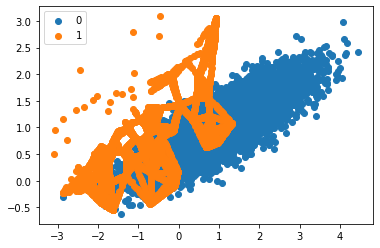
We can notice that the synthetic sample generation is focused around the decision boundary as the region has the low density
Note: Each of the SMOTE variants performs differently depending on the spread of data however just like in borderline smote or in adasyn when synthetic classes overlap each other tend to have low accuracy in the model output. So based on the data we can compare and use the SMOTE variant that gives the best performance.
Moving Ahead there is an again another small method to treat the imbalanced class dataset called NEAR MISS which we will discuss in my next article, wanna keep the article short and clean.
See you there!
Some of my alternative internet presences are Facebook, Instagram, Udemy, Blogger, Issuu, and more.
Also available on Quora @ https://www.quora.com/profile/Rupak-Bob-Roy
Have a good day.


Comments
Post a Comment