Ethereum Fraud Detection.

April 12, 2022

Ethereum Fraud Detection.

Hi, it’s been a while haven’t written anything. But I’m back with some cool data to apply machine learning with. It’s Ethereum transactional dataset where we will create a model to identify fraud detection in the cryptocurrency world. You can download the dataset from here @ github.com/rupak-roy

I will try to keep it short and simple neat and clean with a few advance techniques like automation of best model selection.

Shall we get started?

import pandas as pd
dataset = pd.read_csv("transaction_dataset.csv",sep=",")

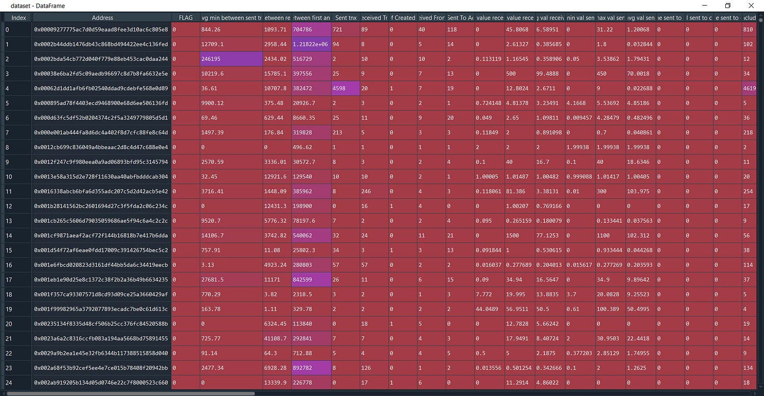
This dataset contains rows of known fraud and valid transactions made over Ethereum.

Here is a description of the rows of the dataset:

--Index: the index number of a row
--Address: the address of the ethereum account
--FLAG: whether the transaction is fraud or not
--Avg min between sent tnx: Average time between sent transactions for account in minutes.
--Avgminbetweenreceivedtnx: Average time between received transactions for account in minutes
--TimeDiffbetweenfirstand_last(Mins): Time difference between the first and last transaction.
--Sent_tnx: Total number of sent normal transactions.
--Received_tnx: Total number of received normal transactions.
--NumberofCreated_Contracts: Total Number of created contract transactions.
--UniqueReceivedFrom_Addresses: Total Unique addresses from which account received transactions.
---UniqueSentTo_Addresses20: Total Unique addresses from which account sent transactions.
--MinValueReceived: Minimum value in Ether ever received.
--AvgValueReceived5Average value in Ether ever received.
--MinValSent: Minimum value of Ether ever sent.
--AvgValSent: Average value of Ether ever sent.
--MinValueSentToContract: Minimum value of Ether sent to a contract
--AvgValueSentToContract: Average value of Ether sent to contracts.
--MaxValueSentToContract: Maximum value of Ether sent to a contract
--TotalTransactions(IncludingTnxtoCreate_Contract): Total number of transactions
--TotalEtherSent:Total Ether sent for account address
--TotalEtherReceived: Total Ether received for account address
--TotalEtherSent_Contracts: Total Ether sent to Contract addresses
--TotalEtherBalance: Total Ether Balance following enacted transactions
--TotalERC20Tnxs: Total number of ERC20 token transfer transactions
--ERC20TotalEther_Received: Total ERC20 token received transactions in Ether
--ERC20TotalEther_Sent: Total ERC20token sent transactions in Ether
--ERC20TotalEtherSentContract: Total ERC20 token transfer to other contracts in Ether
--ERC20UniqSent_Addr: Number of ERC20 token transactions sent to Unique account addresses
--ERC20UniqRec_Addr: Number of ERC20 token transactions received from Unique addresses.
--ERC20UniqRecContractAddr: Number of ERC20token transactions received from Unique contract addresses.
--ERC20AvgTimeBetweenSent_Tnx: Average time between ERC20 token sent transactions in minutes
--ERC20AvgTimeBetweenRec_Tnx: Average time between ERC20 token received transactions in minutes
--ERC20AvgTimeBetweenContract_Tnx: Average time ERC20 token between sent token transactions
--ERC20MinVal_Rec: Minimum value in Ether received from ERC20 token transactions for account.
--ERC20MaxVal_Rec: Maximum value in Ether received from ERC20 token transactions for account
--ERC20AvgVal_Rec: Average value in Ether received from ERC20 token transactions for account
--ERC20MinVal_Sent: Minimum value in Ether sent from ERC20 token transactions for account
--ERC20MaxVal_Sent: Maximum value in Ether sent from ERC20 token transactions for account
--ERC20AvgVal_Sent: Average value in Ether sent from ERC20 token transactions for account
--ERC20UniqSentTokenName: Number of Unique ERC20 tokens transferred
--ERC20UniqRecTokenName: Number of Unique ERC20 tokens received
--ERC20MostSentTokenType: Most sent token for account via ERC20 transaction
--ERC20MostRecTokenType: Most received token for account via ERC20 transactions

Long List! ha.

let’s load the required packages.

#etherum fraud detection

import pandas as pd
import numpy as np
import seaborn as sns
import math
import matplotlib.pyplot as plt

from sklearn import metrics
from sklearn.metrics import classification_report, confusion_matrix
from sklearn.model_selection import cross_val_score
from sklearn.model_selection import KFold

from numpy import mean
from numpy import std
from sklearn.model_selection import RepeatedStratifiedKFold
from sklearn.linear_model import LogisticRegression
from sklearn.neighbors import KNeighborsClassifier
from sklearn.tree import DecisionTreeClassifier
from sklearn.ensemble import RandomForestClassifier
from sklearn.svm import SVC
from sklearn.naive_bayes import GaussianNB

Now select the columns as IV’s and replace the spaces in column names

dataset = dataset.iloc[:,2:]

dataset.columns = dataset.columns.str.replace(' ', '')

We will look for options if there is a way to group either by Address or any

#checking if we can group
from collections import Counter
len(Counter(dataset.Address))

def counts (data):
    counts = Counter(data)
    print(counts)
    print("length",len(counts))

counts(dataset.Address)
counts(dataset.ERC20_most_rec_token_type)
counts(dataset.ERC20mostsenttokentype)

d =dataset.groupby(dataset.ERC20mostsenttokentype).mean()

Split the grouped data into X and y

X = d.iloc[:,1:]
X.isna().any()
#found no missing values

y =  d["FLAG"]
y = np.round(y).astype(int)
y.groupby(y).size()
#Class imbalance
FLAG
0    261
1     44

Remove the multi-collinearity

# Create correlation matrix
corr_matrix = X.corr().abs()

#------Remove the higly correlated variables-------------------
# Select upper triangle of correlation matrix
upper = corr_matrix.where(np.triu(np.ones(corr_matrix.shape), k=1).astype(np.bool))
# Find features with correlation greater than 0.95
to_drop = [column for column in upper.columns if any(upper[column] > 0.70)]
# Drop features 
X.drop(to_drop, axis=1, inplace=True)

#Drop columns that have 1 unique value -------------------------
X.loc[:,X.nunique()!=1]
X.drop(columns=X.columns[X.nunique()==1], inplace=True)

X = X.values

Almost there our Basic Data-Preprocessing is done!

def evaluation_score (y_test,y_pred):
    cm = confusion_matrix(y_test,y_pred) 
    print("Confusion Matrix \n", cm)
    print('Balanced Accuracy ',metrics.balanced_accuracy_score(y_test,y_pred))
    print("Recall Accuracy Score~TP",metrics.recall_score(y_test, y_pred))
    print("Precision Score ~ Ratio of TP",metrics.precision_score(y_test, y_pred))
    print("F1 Score",metrics.f1_score(y_test, y_pred))
    print("auc_roc score", metrics.roc_auc_score(y_test,y_pred))
    print("Classification Report", classification_report(y_test,y_pred))
    
    
def cross_validation(model,X_train,y_train,n):
    kfold = KFold(n_splits=10)  
    accuracies = cross_val_score(model,X= X_train,y= y_train,cv = kfold,scoring='accuracy')
    print("Standard Deviation",accuracies.std())
    print("Mean/Average Score",accuracies.mean())

The functions above will help us give the accuracy scores of the model in just one shot rather than writing over and over again!

from sklearn.preprocessing import StandardScaler
sc = StandardScaler()
X = sc.fit_transform(X)

from sklearn.model_selection import train_test_split
X_train, X_test, y_train, y_test = train_test_split(X,y, test_size = 0.3, random_state = 0)

from sklearn.ensemble import RandomForestClassifier
rf_model = RandomForestClassifier(n_estimators= 150,max_depth=100)
rf_model.fit(X_train,y_train)
y_pred = rf_model.predict(X_test)

Normalize the magnitude of data with StandardScaler() then split the dataset into train and test.

#Accuracy Score

evaluation_score(y_test, y_pred)

Confusion Matrix 
 [[81  5]
 [ 0  6]]
Balanced Accuracy  0.9709302325581395
Recall Accuracy Score~TP 1.0
Precision Score ~ Ratio of TP 0.5454545454545454
F1 Score 0.7058823529411764
auc_roc score 0.9709302325581396
Classification Report               
       precision    recall  f1-score   support

0       1.00      0.94      0.97        86
1       0.55      1.00      0.71         6

accuracy                           0.95        92
   macro avg       0.77      0.97      0.84        92
weighted avg       0.97      0.95      0.95        92

#-----------------------------------------------------------
cross_validation(rf_model,X_train,y_train,10)

Standard Deviation 0.05420814068426065
Mean/Average Score 0.9106060606060605

We have achieved a great score in our first trial without any tuning. Now let’s create syntactic data to tackle the class imbalance issue and see if we can improve our accuracy. Becoz you know the above model with imbalanced class is misleading the model accuracy, it's like the model is more train to identify one class rather than both.

#----------- WITH SMOTE-------------------------------

y 
X

# describes info about train and test set 
print("Number transactions X_train dataset: ", X_train.shape) 
print("Number transactions y_train dataset: ", y_train.shape) 
print("Number transactions X_test dataset: ", X_test.shape) 
print("Number transactions y_test dataset: ", y_test.shape)

Number transactions X_train dataset: (213, 45)
Number transactions y_train dataset: (213,)
Number transactions X_test dataset: (92, 45)
Number transactions y_test dataset: (92,)

from imblearn.over_sampling import SMOTE

print("Before OverSampling, counts of label '1': {}".format(sum(y_train == 1))) 
print("Before OverSampling, counts of label '0': {} \n".format(sum(y_train == 0)))

# import SMOTE module from imblearn library 
# pip install imblearn (if you don't have imblearn in your system) 
from imblearn.over_sampling import SMOTE 
sm = SMOTE(random_state = 2,sampling_strategy=1) 
X_train_res, y_train_res = sm.fit_resample(X_train, y_train.ravel())

print('After OverSampling, the shape of train_X: {}'.format(X_train_res.shape)) 
print('After OverSampling, the shape of train_y: {} \n'.format(y_train_res.shape))

print("After OverSampling, counts of label '1': {}".format(sum(y_train_res == 1))) 
print("After OverSampling, counts of label '0': {}".format(sum(y_train_res == 0)))

Before OverSampling, counts of label ‘1’: 38
Before OverSampling, counts of label ‘0’: 175

After OverSampling, the shape of train_X: (350, 45)
After OverSampling, the shape of train_y: (350,)

After OverSampling, counts of label ‘1’: 175
After OverSampling, counts of label ‘0’: 175

Have our class balanced, Time to apply our model with our new data

def train_model(n,max_d):
    rf_model =RandomForestClassifier(n_estimators=n,  
     max_depth=max_d)
    rf_model.fit(X_train_res,y_train_res.ravel())
    predictions = rf_model.predict(X_test)
    return predictions

def show_predictions(data):
    results = rf_model.predict(data)
    return results 
    
    
train_model_predictions = train_model(500,100)

Get the accuracy Score

#Accuracy Score--------------------------------------

evaluation_score(y_test, train_model_predictions)

Confusion Matrix 
 [[79  7]
 [ 0  6]]
Balanced Accuracy  0.9593023255813953
Recall Accuracy Score~TP 1.0
Precision Score ~ Ratio of TP 0.46153846153846156
F1 Score 0.631578947368421
auc_roc score 0.9593023255813953
Classification Report               
       precision    recall  f1-score   support

0       1.00      0.92      0.96        86
1       0.46      1.00      0.63         6

accuracy                           0.92        92
   macro avg       0.73      0.96      0.79        92
weighted avg       0.96      0.92      0.94        92

#----------------------------------------------------------

cross_validation(rf_model,X_train,y_train,10)

Standard Deviation 0.04696321299032405
Mean/Average Score 0.8965367965367965

Might be wondering we are down by 0.2 % accuracy. Well, that's becoz i use n_estimators =500. Chill!

Now as promised in the beginning will show you a way to identify the algorithm that will perform best from the rest

#Select the best model----------------------------------------
def get_models():
    models = dict()
    models['lr'] = LogisticRegression()
    models['knn'] = KNeighborsClassifier()
    models['cart'] = DecisionTreeClassifier()
    models['svm'] = SVC()
    models['random_forest'] = RandomForestClassifier()
    models['bayes'] = GaussianNB()
    return models

# evaluate a give model using cross-validation
def evaluate_model(model, X, y):
 cv = RepeatedStratifiedKFold(n_splits=10, n_repeats=3, random_state=1)
 scores = cross_val_score(model, X, y, scoring='accuracy', cv=cv, n_jobs=-1, error_score='raise')
 return scores

# get the models to evaluate
models = get_models()
# evaluate the models and store results
results, names = list(), list()
for name, model in models.items():
 scores = evaluate_model(model, X, y)
 results.append(scores)
 names.append(name)
 print('>%s %.3f (%.3f)' % (name, mean(scores), std(scores)))
# plot model performance for comparison
plt.boxplot(results, labels=names, showmeans=True)
plt.show()

Run the loop and you will get the plot below.

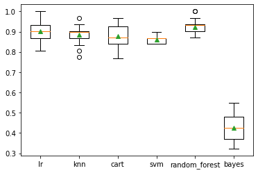
From the plot, we can clearly observe the baseline models where Random Forest and the logistic regression are performing the best.

Now it becomes easier to select algorithms and start working with it.

#GridSeachCV -----
from sklearn.model_selection import GridSearchCV

p = [{'n_estimators':[50,100,150],'max_depth':[10, 100]}]

grid_search = GridSearchCV(estimator = rf_model,param_grid= p, scoring = "accuracy",cv=10,n_jobs=-1)
grid_search = grid_search.fit(X_train,y_train)

best_accuracy = grid_search.best_score_
best_parameters = grid_search.best_params_
print("best accuracy , best_paramters", best_accuracy, best_parameters)

best accuracy =0.9203463203463202, best_paramters {‘max_depth’: 10, ‘n_estimators’: 100}

We have our tuned parameters of random forest, Fit it and good to go!

train_model_predictions1= train_model(100,10)

#Accuracy Score
evaluation_score(y_test, train_model_predictions1)
cross_validation(rf_model,X_train,y_train,10)

show_predictions(X_test)

Let’s me put of the pieces together so that you can also use it

#etherum fraud detection

import pandas as pd
import numpy as np
import seaborn as sns
import math
import matplotlib.pyplot as plt

from sklearn import metrics
from sklearn.metrics import classification_report, confusion_matrix
from sklearn.model_selection import cross_val_score
from sklearn.model_selection import KFold

from numpy import mean
from numpy import std
from sklearn.model_selection import RepeatedStratifiedKFold
from sklearn.linear_model import LogisticRegression
from sklearn.neighbors import KNeighborsClassifier
from sklearn.tree import DecisionTreeClassifier
from sklearn.ensemble import RandomForestClassifier
from sklearn.svm import SVC
from sklearn.naive_bayes import GaussianNB

dataset = pd.read_csv("transaction_dataset.csv",sep=",")
dataset = dataset.iloc[:,2:]

dataset.columns = dataset.columns.str.replace(' ', '')

#checking if we can group
from collections import Counter
len(Counter(dataset.Address))

def counts (data):
    counts = Counter(data)
    print(counts)
    print("length",len(counts))

counts(dataset.Address)
counts(dataset.ERC20_most_rec_token_type)
counts(dataset.ERC20mostsenttokentype)

d =dataset.groupby(dataset.ERC20mostsenttokentype).mean()

X = d.iloc[:,1:]
y =  d["FLAG"]
y = np.round(y).astype(int)
y.groupby(y).size()
#Class imbalance issue

X.isna().any()

def outlier_dec(data):
    sns.boxplot(data)
    
outlier_dec(X.Avgminbetweensenttnx)

#----------------------------------------------------------

# Create correlation matrix
corr_matrix = X.corr().abs()

#------Remove the highly correlated variables----------------------
# Select upper triangle of correlation matrix
upper = corr_matrix.where(np.triu(np.ones(corr_matrix.shape), k=1).astype(np.bool))
# Find features with correlation greater than 0.95
to_drop = [column for column in upper.columns if any(upper[column] > 0.70)]
# Drop features 
X.drop(to_drop, axis=1, inplace=True)

#Drop columns that have 1 unique value -------------------------
X.loc[:,X.nunique()!=1]
X.drop(columns=X.columns[X.nunique()==1], inplace=True)

X = X.values

#----------------------------

def evaluation_score (y_test,y_pred):
    cm = confusion_matrix(y_test,y_pred) 
    print("Confusion Matrix \n", cm)
    print('Balanced Accuracy ',metrics.balanced_accuracy_score(y_test,y_pred))
    print("Recall Accuracy Score~TP",metrics.recall_score(y_test, y_pred))
    print("Precision Score ~ Ratio of TP",metrics.precision_score(y_test, y_pred))
    print("F1 Score",metrics.f1_score(y_test, y_pred))
    print("auc_roc score", metrics.roc_auc_score(y_test,y_pred))
    print("Classification Report", classification_report(y_test,y_pred))
    
    
def cross_validation(model,X_train,y_train,n):
    kfold = KFold(n_splits=10)  
    accuracies = cross_val_score(model,X= X_train,y= y_train,cv = kfold,scoring='accuracy')
    print("Standard Deviation",accuracies.std())
    print("Mean/Avergae Score",accuracies.mean())

#----------------------------

from sklearn.preprocessing import StandardScaler
sc = StandardScaler()
X = sc.fit_transform(X)

from sklearn.model_selection import train_test_split
X_train, X_test, y_train, y_test = train_test_split(X,y, test_size = 0.3, random_state = 0)

from sklearn.ensemble import RandomForestClassifier
rf_model = RandomForestClassifier(n_estimators= 150,max_depth=100)
rf_model.fit(X_train,y_train)
y_pred = rf_model.predict(X_test)

#Accuracy SCore

evaluation_score(y_test, y_pred)

cross_validation(rf_model,X_train,y_train,10)

#----------- WITH SMOTE

y 
X

# describes info about train and test set 
print("Number transactions X_train dataset: ", X_train.shape) 
print("Number transactions y_train dataset: ", y_train.shape) 
print("Number transactions X_test dataset: ", X_test.shape) 
print("Number transactions y_test dataset: ", y_test.shape)

#----------------------------------------------
from imblearn.over_sampling import SMOTE

print("Before OverSampling, counts of label '1': {}".format(sum(y_train == 1))) 
print("Before OverSampling, counts of label '0': {} \n".format(sum(y_train == 0)))

# import SMOTE module from imblearn library 
# pip install imblearn (if you don't have imblearn in your system) 
from imblearn.over_sampling import SMOTE 
sm = SMOTE(random_state = 2,sampling_strategy=1) 
X_train_res, y_train_res = sm.fit_resample(X_train, y_train.ravel())

print('After OverSampling, the shape of train_X: {}'.format(X_train_res.shape)) 
print('After OverSampling, the shape of train_y: {} \n'.format(y_train_res.shape))

print("After OverSampling, counts of label '1': {}".format(sum(y_train_res == 1))) 
print("After OverSampling, counts of label '0': {}".format(sum(y_train_res == 0)))

def train_model(n,max_d):
    rf_model = RandomForestClassifier(n_estimators=n,max_depth=max_d)
    rf_model.fit(X_train_res,y_train_res.ravel())
    predictions = rf_model.predict(X_test)
    return predictions

def show_predictions(data):
    results = rf_model.predict(data)
    return results 
    
    
train_model_predictions = train_model(500,100)

#Accuracy Score--------------------------------------

evaluation_score(y_test, train_model_predictions)
cross_validation(rf_model,X_train,y_train,10)

#Select the best model------------------------------------------
def get_models():
    models = dict()
    models['lr'] = LogisticRegression()
    models['knn'] = KNeighborsClassifier()
    models['cart'] = DecisionTreeClassifier()
    models['svm'] = SVC()
    models['random_forest'] = RandomForestClassifier()
    models['bayes'] = GaussianNB()
    return models

# evaluate a give model using cross-validation
def evaluate_model(model, X, y):
 cv = RepeatedStratifiedKFold(n_splits=10, n_repeats=3, random_state=1)
 scores = cross_val_score(model, X, y, scoring='accuracy', cv=cv, n_jobs=-1, error_score='raise')
 return scores

# get the models to evaluate
models = get_models()
# evaluate the models and store results
results, names = list(), list()
for name, model in models.items():
 scores = evaluate_model(model, X, y)
 results.append(scores)
 names.append(name)
 print('>%s %.3f (%.3f)' % (name, mean(scores), std(scores)))
# plot model performance for comparison
plt.boxplot(results, labels=names, showmeans=True)
plt.show()

#GridSeachCV -----
from sklearn.model_selection import GridSearchCV

p = [{'n_estimators':[50,100,150],'max_depth':[10, 100]}]

'''p = [{'n_estimators':[50,100,150],'max_depth':[10, 100],
               'min_samples_split':[2,3,4,5,6,7,8,9,10],'min_samples_leaf':[2,3,4,5],
               'min_impurity_decrease':[2,3,4,5],'max_features':["auto","sqrt","log2"]}]'''

grid_search = GridSearchCV(estimator = rf_model,param_grid= p, scoring = "accuracy",cv=10,n_jobs=-1)
grid_search = grid_search.fit(X_train,y_train)
best_accuracy = grid_search.best_score_
best_parameters = grid_search.best_params_
print("best accuracy , best_paramters", best_accuracy, best_parameters)
#-------------------------------------------

train_model_predictions1= train_model(100,10)
#Accuracy Score
evaluation_score(y_test, train_model_predictions1)
cross_validation(rf_model,X_train,y_train,10)

show_predictions(new_data)

Next, we have another interesting and advanced hybrid model method specially used for non-linear data

If you like to know more about advanced topics like clustering follow my other article A-Z Clustering

Some of my alternative internet presences are Facebook, Instagram, Udemy, Blogger, Issuu, and more.

Also available on Quora @ https://www.quora.com/profile/Rupak-Bob-Roy

Have a good day.

Search This Blog

Welcome to #bobrupakroy

Ethereum Fraud Detection.

Have a good day.

Comments

Post a Comment

Popular Posts

Near Miss — under sampling

Auto — TS — Ensemble