OPTICS CLUSTERING. Ordering Points To Identify Cluster Structure (OPTICS) ) is a density-based clustering technique that allows partitioning data into groups with similar characteristics(clusters)

Its addresses one of the DBSCAN’s major weaknesses. The problem of detecting meaningful clusters in data of varying density.
In a density based clustering, clusters are defined as dense regions of data points separated by low-density regions.
It adds two more terms to the concepts of DBSCAN clustering. They are:
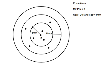
- Core Distance: it is the minimum value of radius required to classify a given point as a core point. if the given point is not a Core point, then its Core Distance is undefined.
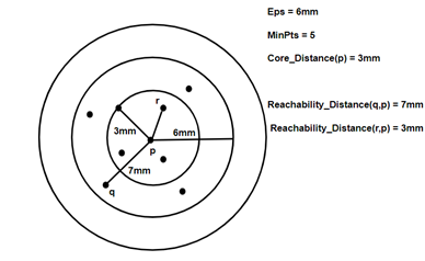
2. Reachability Distance: it is defined with respect to another data point ‘q’. The Reachability distance between a point p and q . Note that The Reachability Distance is not defined if ‘q’ is not a Core point.
Few advantages:
· OPTICS clustering doesn’t require a predefined number of clusters in advance.
· Clusters can be of any shape, including non-spherical ones.
· Able to identify outliers(noise data)
Disadvantages:
· It fails if there are no density drops between clusters.
· It is also sensitive to parameters that define density( radius and the minimum number of points) and proper parameter settings require domain knowledge.
Now let’s understand the coding part.
First, we will load our dataset and perform a few data pre-processing steps like scaling.
#OPTICS Clustering
import numpy as np
import pandas as pd
import matplotlib.pyplot as plt
from matplotlib import gridspec
from sklearn.cluster import OPTICS, cluster_optics_dbscan
from sklearn.preprocessing import normalize, StandardScaler
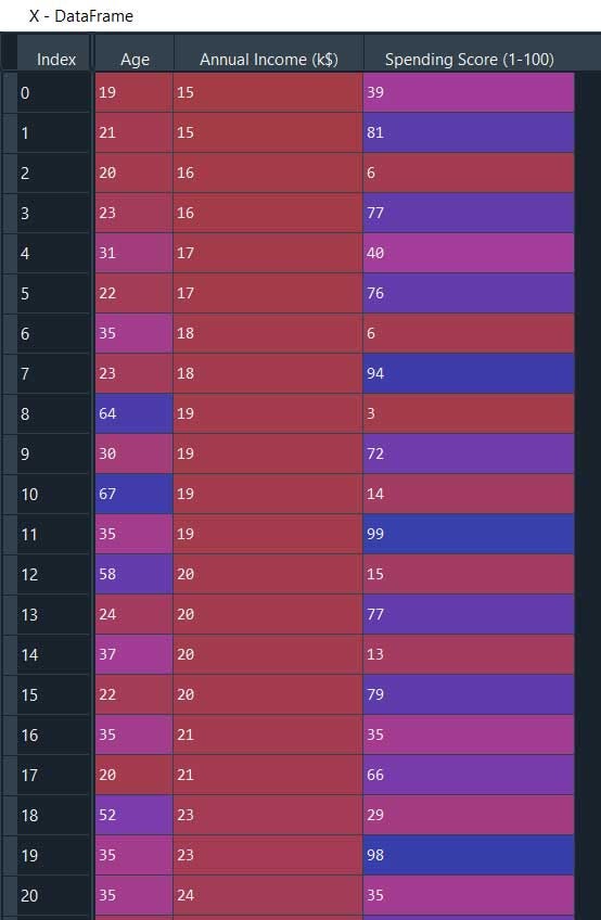
X = pd.read_csv('Mall_Customers.csv')#Dropping irrelevant columns
drop_features = ['CustomerID', 'Genre']
X = X.drop(drop_features, axis = 1)
#Handling the missing values if any
X.fillna(method ='ffill', inplace = True)
X.head()
#Pre-processing of data
#Scaling the data to bring all the attributes to a comparable level
scaler = StandardScaler()
X_scaled = scaler.fit_transform(X)
#Normalizing the data so that the data
#approximately follows a Gaussian distribution
X_normalized = normalize(X_scaled)
#Converting the numpy array into a pandas DataFrame
X_normalized = pd.DataFrame(X_normalized)
#Renaming the columns
X_normalized.columns = X.columns
X_normalized.head()
Now we will build the model using min_samples = 10, xi =0.05, min_cluster_size = 0.05
#Building the OPTICS Clustering model
optics_model = OPTICS(min_samples = 10, xi = 0.05, min_cluster_size = 0.05)
'''xi:float, between 0 and 1, optional (default=0.05)
Determines the minimum steepness on the reachability plot that constitutes a cluster boundary.
For example, an upwards point in the reachability plot is defined by the ratio from one point
to its successor being at most 1-xi. Used only when cluster_method='xi'.
'''
#Training the model
optics_model.fit(X_normalized)
Here we are..our OPTICS model is complete…. We can print the cluster labels using optics_model.labels_
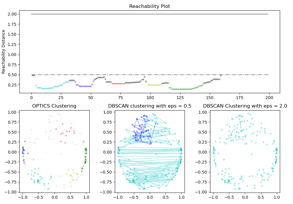
Now we will take one step further by comparing the performance of OPTICS and DBSCAN to validate DBSCAN lacks clustering in different densities
#Producing the labels according to the DBSCAN technique with eps = 0.5
labels1 = cluster_optics_dbscan(reachability = optics_model.reachability_,
core_distances = optics_model.core_distances_,ordering = optics_model.ordering_, eps = 0.5)
#Producing the labels according to the DBSCAN technique with eps = 2.0
labels2 = cluster_optics_dbscan(reachability = optics_model.reachability_,
core_distances = optics_model.core_distances_,
ordering = optics_model.ordering_, eps = 2)
#Creating a numpy array with numbers at equal spaces till
#the specified range
space = np.arange(len(X_normalized))
#Storing the reachability distance of each point
reachability = optics_model.reachability_[optics_model.ordering_]
#Visualizing the results
#Defining the framework of the visualization
plt.figure(figsize =(10, 7))
G = gridspec.GridSpec(2, 3)
ax1 = plt.subplot(G[0, :])
ax2 = plt.subplot(G[1, 0])
ax3 = plt.subplot(G[1, 1])
ax4 = plt.subplot(G[1, 2])
#Plotting the Reachability-Distance Plot
colors = ['c.', 'b.', 'r.', 'y.', 'g.']
for Class, colour in zip(range(0, 5), colors):
Xk = space[labels == Class]
Rk = reachability[labels == Class]
ax1.plot(Xk, Rk, colour, alpha = 0.3)
ax1.plot(space[labels == -1], reachability[labels == -1], 'k.', alpha = 0.3)
ax1.plot(space, np.full_like(space, 2., dtype = float), 'k-', alpha = 0.5)
ax1.plot(space, np.full_like(space, 0.5, dtype = float), 'k-.', alpha = 0.5)ax1.set_ylabel('Reachability Distance')
ax1.set_title('Reachability Plot')
#Plotting the OPTICS Clustering
colors = ['c.', 'b.', 'r.', 'y.', 'g.']
for Class, colour in zip(range(0, 5), colors):
Xk = X_normalized[optics_model.labels_ == Class]
ax2.plot(Xk.iloc[:, 0], Xk.iloc[:, 1], colour, alpha = 0.3)
ax2.plot(X_normalized.iloc[optics_model.labels_ == -1, 0],
X_normalized.iloc[optics_model.labels_ == -1, 1],'k+', alpha = 0.1)
ax2.set_title('OPTICS Clustering')
#Plotting the DBSCAN Clustering with eps = 0.5
colors = ['c', 'b', 'r', 'y', 'g', 'greenyellow']
for Class, colour in zip(range(0, 6), colors):
Xk = X_normalized[labels1 == Class]
ax3.plot(Xk.iloc[:, 0], Xk.iloc[:, 1], colour, alpha = 0.3, marker ='.')
ax3.plot(X_normalized.iloc[labels1 == -1, 0],X_normalized.iloc[labels1 == -1, 1],'k+', alpha = 0.1)
ax3.set_title('DBSCAN clustering with eps = 0.5')
#Plotting the DBSCAN Clustering with eps = 2.0
colors = ['c.', 'y.', 'm.', 'g.']
for Class, colour in zip(range(0, 4), colors):
Xk = X_normalized.iloc[labels2 == Class]
ax4.plot(Xk.iloc[:, 0], Xk.iloc[:, 1], colour, alpha = 0.3)
ax4.plot(X_normalized.iloc[labels2 == -1, 0], X_normalized.iloc[labels2 == -1, 1],'k+', alpha = 0.1)
ax4.set_title('DBSCAN Clustering with eps = 2.0')plt.tight_layout()
plt.show()
Next, we have another interesting and advanced clustering method specially used for data exploration and visualizing high-dimensional data called T-SNE.
If you like to know more about advanced types of clustering follow my other article A-Z Clustering
Some of my alternative internet presences are Facebook, Instagram, Udemy, Blogger, Issuu, and more.
Also available on Quora @ https://www.quora.com/profile/Rupak-Bob-Roy
Have a good day.


Comments
Post a Comment