A-Z Clustering. ~ Full Guide to 15 different types of clustering methods.
Hi there whatsup? I hope it's all good!
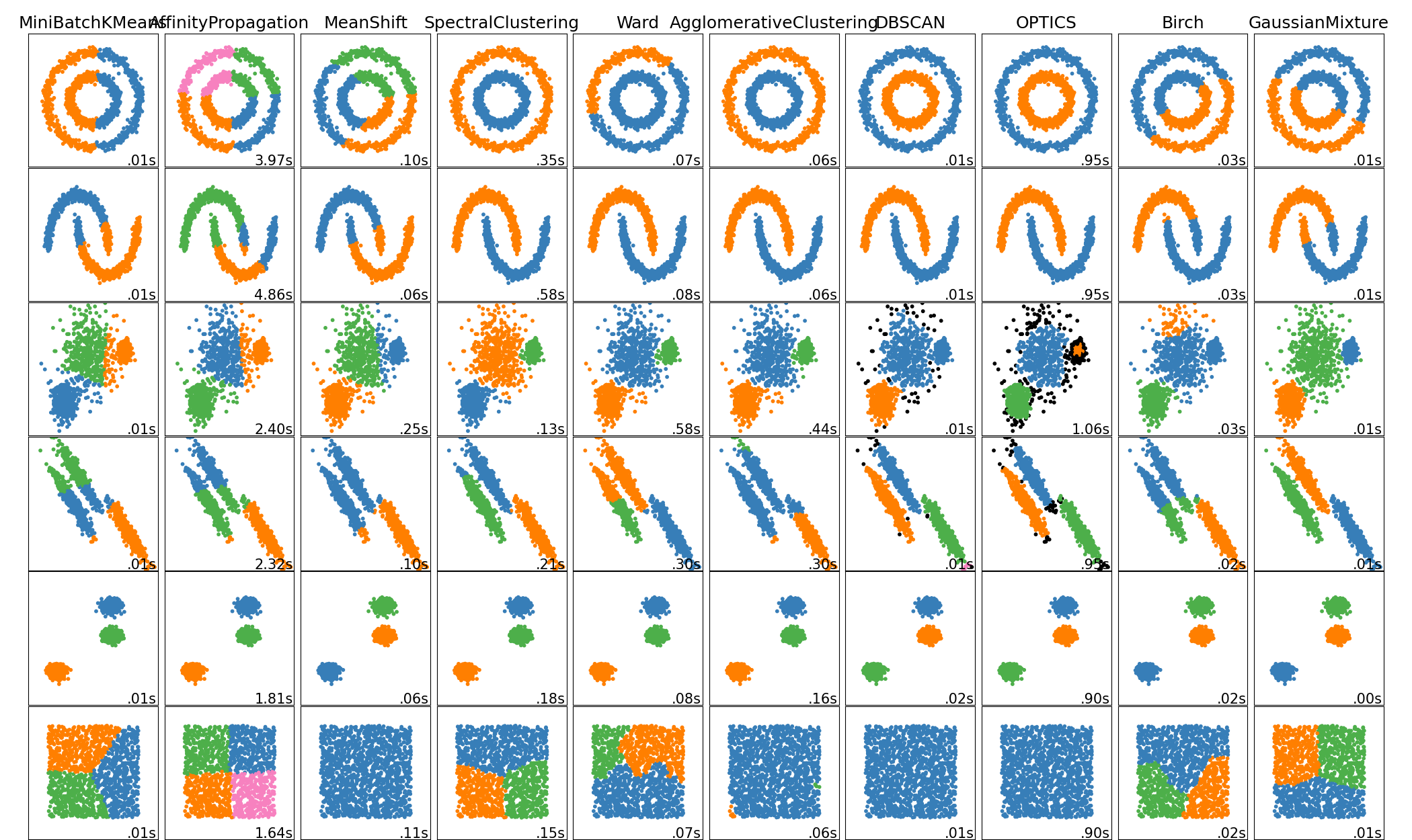
Today we will take clustering into another level with more than 12 types of clustering methods.
It's gonna be a long chapter, shall we get started?
Here are the lists of clustering techniques that we will be going through:
1.) K-means
2.) H-Clust
3.) DBSCAN / Density-Based Spatial Clustering
4.) HDBSCAN / Hierarchical Density-Based Spatial Clustering
5.) Cure Algorithm
6.) Mini-Batch K-means Clustering
7.) Fuzzy Clustering
8.) Spectral Clustering
9.) Mean Shift
10.) BRICH / Balanced Iterative Reducing and Clustering using Hierarchies
11.) K-Mediod
12.) Optics Clustering
13.) T-SNE / T-distributed Stochastic Neighbor Embedding Clustering
14.) Sub Space Clustering
15.) Chameleon Clustering (coming soon)
16.) Cluster Evaluation
First, let’s start with K-means Clustering, The Widely used isn’t it?
What is clustering? Clustering is a process of grouping a set of observations that the same group is similar to each other than to those of others within a large population. Example Types of car sub, sedan, sports, economic, etc.
Steps for performing clustering.
1st determine the number of clusters i.e. Values of ‘K’
2nd now the algorithm will assign the observations/clusters to the seeds based on their close proximity.
Now how the algorithm will decide which observation is closed to which seed either the left or right seed?
3rd for that draw a perpendicular bisector between the lines from the mid-point.
So any point to the left is closer to seed1(cluster) & any point to the right is closer to seed 2 (cluster)
Similarly when we draw a perpendicular() to seed 3 and any point to the above is closer to seed 3 & any point to the below is closer to seed 1
4th and the algorithm will create groups i.e. the clusters. But how do we know these are the most optimal clusters based on the seeds. It calculates the centroid of these clusters i.e. mid-points which is calculated by averaging the midpoints of each cluster. This is how K-means of clustering technique works.
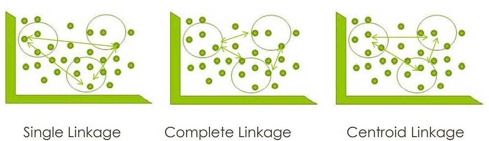
3 Methods to calculate the distance
1.) Single Linkage: The distance between 2 clusters is determined by the distance between eh closet members of those 2 clusters.
2.) Complete Linkage: in complete linkage, the distance is given by the most distance between the closet members of the 2 clusters.
3.) Centroid Linkage: in centroid linkage, the distance between centroids that is the mid-points of the clusters are used to determine the distance between clusters.
Data Preparation for clustering
- Scaling: is a concept of bringing together different measures of variables into one uniform scale of measure. In other words, maintaining a uniform identity to understand the variance between them.
Because the algorithm will think it is a variance rather than a different scale of measure. So in order to do effective clustering, we need to adjust the variable to a common scale
= Scaled between (0–1)
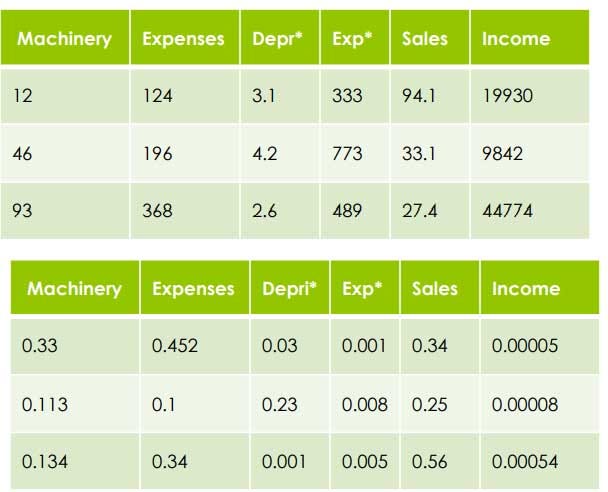
4 Methods of Scaling
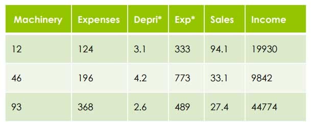
- Divide each variable by the range after subtracting the lowest Example: Machinery Highest = 93
Lowest = 12
Range = 93–12 = 81
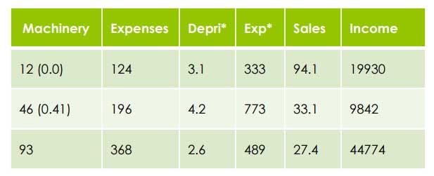
Divide each variable by the range after subtracting the lowest
=> 12–12/81=0.0 => 46–12/81=34/81=0.41
2. Divide each variable by the mean of the variable Example: Machinery Mean= 50.33
=> 12/50.33= 0.28
=> 46/50.33= 0.91
3. Normalization / Z scoring of variables (commonly used appropriate method)
— Subtract mean from each variable then divide by standard deviation Example: Machinery
Variable1 — mean/standard deviation=12–50.33/40.67 = -0.94
Variable1 — mean/standard deviation=46–50.33/40.67 = -0.11
Weighing: concept of adjusting the values of the variable as per their relative importance.
The first step before weighing is to scale all the variables & standardize them. Now we can tell the algorithm which variables are more important than the others.
For example, if we assign a weight of 2 to a variable product category after having them on a common scale then we will just multiply X-times ( like multiplied by 3) in order to generate a new weighted variable.
4. Others: There are many other ways to scale the data without disturbing the variance, once such is Logarithm by converting the values in the log which also ranges from 0 to 1
Don‟t worry we won‟t be manually calculating each of them instead we will use functions that will do the scaling for us.
Handling Categorical Data
Clustering algorithms can handle continuous data.
But what if it contains Categorical Data Types like
Nominal (no order)
Furniture A VS Furniture B
High vs Med vs Low
Ordinal
Tea VS Coffee Rating: 1 to 5, Yes vs No
So the easiest way to solve this is to create Binary Variables
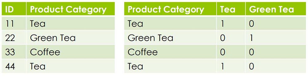
Binary Variables are also a type of Categorical Variables but it is in 0,1binary format. Therefore it can be handled by the clustering algorithm.
Evaluating Clusters
- The difference in Centroid Average distance between the cluster centroids divided by the average distance between the members and the cluster centroid
- 2. Profiling Clusters Profiling is another way to identify each cluster & why it is different from the rest. For example, take the mean of each variable within the cluster & compare it to the mean of the same variable of the population. Here too I will show you another way to evaluate the clusters using special packages and functions.
Since there is no target variable in clustering it can be highly used to identify hidden patterns in the data without any hypothesis. It can also be categorized as Unsupervised Machine Learning
Some of the few use cases of clustering are Segmentation like Customer, Product Segmentation, Outlier Detection or Fraud Detection, or Improving the performance of the other techniques by segmenting the data into smaller groups
Improving Clusters: in case if we have one or a few strong clusters, remove the strong cluster and recalculate the cluster from the remaining to detect new clusters.
Now let's get some hands-on experience of K-means clustering with the help of an example. For this example we will take a common widely used dataset crime_data.csv
First, let’s import the libraries and the dataset
#Importing the libraries
import numpy as np
import matplotlib.pyplot as plt
import pandas as pd
#Importing the dataset
dataset = pd.read_csv('crime_data.csv')
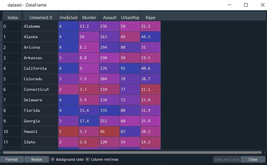
Then we do some data pre-processing like removing rows that have ‘na’ values also we will take from the 3rd column as the 2nd column value have the cluster values.
We can also perform scaling using the StandardScaler function to normalize the magnitude of spread, that is to bring all the values to a range.
Our Data Pre-processing step is complete.
Now it's time to fit /create our model and predict.
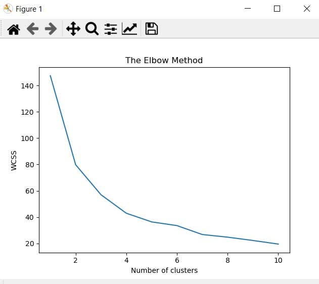
But before that let's get the optimal number of clusters for our model using the elbow method.
#Splitting the dataset into the Training set and Test set
#Here we dont have a dependent variable becoz its an unsupervised #learning so its not required However we will split the data to test #our model with new data
from sklearn.model_selection import train_test_split
X_train, X_test = train_test_split(X, test_size = 0.2, random_state = 0)
#Using the elbow method to find the optimal number of clusters
from sklearn.cluster import KMeans
wcss = []
for i in range(1, 11):
kmeans = KMeans(n_clusters = i, init = 'k-means++', random_state = 0)
kmeans.fit(X_train)
wcss.append(kmeans.inertia_)
plt.plot(range(1, 11), wcss)
plt.title('The Elbow Method')
plt.xlabel('Number of clusters')
plt.ylabel('WCSS')
plt.show()
#Fitting K-Means to the dataset
kmeans_model = KMeans(n_clusters = 4, init = 'k-means++', random_state = 0)
A short note: What is Kmeans & K-means++ as far I know K-means picks the initial centers randomly since they’re based on pure luck, they can be selected really badly.
The K-means++ algorithm tries to solve this problem by spreading the initial centers evenly.
K-means starts with allocating cluster centers randomly and then looks for a “better solution”. K-means++ starts with allocation one cluster center randomly and the searches for other centers given the first one.
According to the wiki. K-means++ usually converges in 2 or 3 iterations and often twice as fast as the standard K-means algorithm.
Alright, we have our K-means model ready. Now it's time to predict.
#Predicting with new data
y_kmeans = kmeans_model.fit_predict(X_train)
y_kmeans1 = kmeans_model.fit_predict(X_test)
here we are X_train containing 80% of our data and X_test containing 20% of our data. Now we can merge the results: clusters for later analysis
Remember for the sake of this example we split the dataset into 2 train and test for you to understand its reusability for various scenarios. However note that we run our model in 80% of data means it will cluster based on that 80% of data off-course but if we add 20% more the clustering results would been different.
#row bind (optional)
results = pd.concat([df,df1])
results.columns = ['Murder','Assault','UrbanPop','Rape','cluster']
#reseting the index value
df.reset_index(drop=True)
Alright let’s see/predict what will the cluster if we have random input
y_kmeans = kmeans_model.fit_predict([[912,64.1]])
#else------------
q=pd.DataFrame([[912,64.1]])
y_kmeans = kmeans_model.fit_predict(q)
This will throw ValueError: n_samples=1 should be >= n_clusters=5 becoz here the single row of data ‘q’ i.e. n_samples = 1 Thus we need data(rows) having n_cluster =4
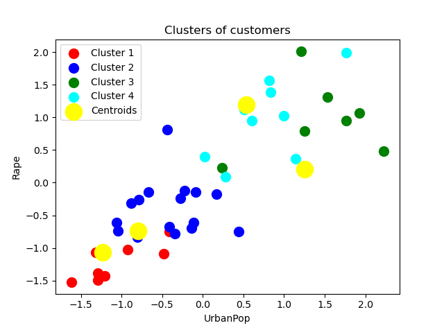
#Visualising the clusters
plt.scatter(X_train[y_kmeans == 0, 0], X_train[y_kmeans == 0, 1], s = 100, c = 'red', label = 'Cluster 1')
plt.scatter(X_train[y_kmeans == 1, 0], X_train[y_kmeans == 1, 1], s = 100, c = 'blue', label = 'Cluster 2')
plt.scatter(X_train[y_kmeans == 2, 0], X_train[y_kmeans == 2, 1], s= 100, c = 'green', label = 'Cluster 3')
plt.scatter(X_train[y_kmeans == 3, 0], X_train[y_kmeans == 3, 1], s = 100, c = 'cyan', label = 'Cluster 4')
plt.scatter(kmeans_model.cluster_centers_[:, 0], kmeans_model.cluster_centers_[:, 1], s = 300, c = 'yellow', label = 'Centroids')
plt.title('Clusters of customers')
plt.xlabel('UrbanPop')
plt.ylabel('Rape')
plt.legend()
plt.show()
Let me put all of the pieces together.
# K-Means Clustering
#Importing the libraries
import numpy as np
import matplotlib.pyplot as plt
import pandas as pd
#Importing the dataset
dataset = pd.read_csv('crime_data.csv')
#drop the missing values
dataset = dataset.dropna()
X = dataset.iloc[:,2:].values
#Normalization
from sklearn.preprocessing import StandardScaler
sc_X = StandardScaler()
X=sc_X.fit_transform(X)
#Splitting the dataset into the Training set and Test set
#Here we dont have a dependent variable becoz its an unsupervised #learning so its not required However we will split the data to test #our model with new data
from sklearn.model_selection import train_test_split
X_train, X_test = train_test_split(X, test_size = 0.2, random_state = 0)
#Using the elbow method to find the optimal number of clusters
from sklearn.cluster import KMeans
wcss = []
for i in range(1, 11):
    kmeans = KMeans(n_clusters = i, init = 'k-means++', random_state = 0)
    kmeans.fit(X_train)
    wcss.append(kmeans.inertia_)
plt.plot(range(1, 11), wcss)
plt.title('The Elbow Method')
plt.xlabel('Number of clusters')
plt.ylabel('WCSS')
plt.show()
#Fitting K-Means to the dataset
kmeans_model = KMeans(n_clusters = 4, init = 'k-means++', random_state = 0)
#Predicting with new data
y_kmeans = kmeans_model.fit_predict(X_train)
y_kmeans1 = kmeans_model.fit_predict(X_test)
#We can also merge the results: clusters for later analysis
df = pd.DataFrame( X_train, y_kmeans)
#renaming the index column
df.index.name = "cluster"
df
#converting index value to columns
df.reset_index(inplace=True)
df1 = pd.DataFrame(X_test,y_kmeans1)
df1.index.name = "cluster"
df1.reset_index(inplace=True)
df1
#row bind (optional)
results = pd.concat([df,df1])
results.columns = ['Murder','Assault','UrbanPop','Rape','cluster']
#reseting the index value
df.reset_index(drop=True)
y_kmeans = kmeans_model.fit_predict([[912,64.1]])
q=pd.DataFrame([[912,64.1]])
y_kmeans = kmeans_model.fit_predict(q)
#this will throw ValueError: n_samples=1 should be >= n_clusters=5 becoz
#here the single row of data i.e. n_samples = 1 Thus we need data(rows) having n_cluster =5
# Visualising the clusters
plt.scatter(X_train[y_kmeans == 0, 0], X_train[y_kmeans == 0, 1], s = 100, c = 'red', label = 'Cluster 1')
plt.scatter(X_train[y_kmeans == 1, 0], X_train[y_kmeans == 1, 1], s = 100, c = 'blue', label = 'Cluster 2')
plt.scatter(X_train[y_kmeans == 2, 0], X_train[y_kmeans == 2, 1], s = 100, c = 'green', label = 'Cluster 3')
plt.scatter(X_train[y_kmeans == 3, 0], X_train[y_kmeans == 3, 1], s = 100, c = 'cyan', label = 'Cluster 4')
plt.scatter(kmeans_model.cluster_centers_[:, 0], kmeans_model.cluster_centers_[:, 1], s = 300, c = 'yellow', label = 'Centroids')
plt.title('Clusters of customers')
plt.xlabel('UrbanPop')
plt.ylabel('Rape')
plt.legend()
plt.show()
We still have a long list to go, lets move on with the next widely used clustering method is hierarchical clustering
Also known as hierarchical cluster analysis which seeks to build a hierarchy of clusters.
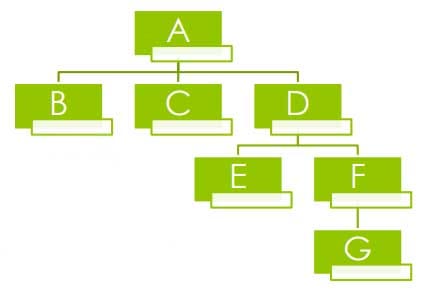
Generally, it is of two types: › a.) Agglomerative: This is a “bottom-up” approach where each observation starts in its own cluster, and pairs of clusters are merged as one moves up the hierarchy. ›
b.) Divisive: This is a “top-down” approach: all observations start in one cluster, and splits are performed recursively as one moves down the hierarchy.
And the most commonly used hierarchical clustering technique is the Agglomerative “ bottom-up” approach.
In K- means clustering we need only scaled data however in hierarchical clustering we need scaled data as well as the distance between two observations.
To calculate the distance we will use Euclidean metric
Then we use certain algorithms in order to handle the types of data for hierarchical clustering:
Ordinal data where data is represented as the value of orders, for example, A customer was asked in a survey to rate the Product After Sales on a scale of 5 to 1, in simple words, ordinal data simply express an order. To handle this type of ordinal data Preferred clustering method is the Single Linkage Method
Interval data where data expresses the difference between 2 values are same, for example, the speed of a car 100mph = 160kph, the temperature in Fahrenheit is the same Celsius. In simple words, it depicts the same magnitude. So to handle this type of Interval data Preferred clustering methods is Complete and Average Linkage Method
Alright, let build our hierarchical cluster.
First as usual we will load the libraries, dataset, scale the data then data pre-processing.
#Importing the libraries
import numpy as np
import matplotlib.pyplot as plt
import pandas as pd
#Importing the dataset
dataset = pd.read_csv('crime_data.csv')
#drop the missing values
dataset = dataset.dropna()
X = dataset.iloc[:,2:].values
#Normalization
from sklearn.preprocessing import StandardScaler
sc_X = StandardScaler()
X=sc_X.fit_transform(X)
#Splitting the dataset into the Training set and Test set
#Here we dont have a dependent variable becoz its an unsupervised learning so its not required However we will split the data to test our model with new data
from sklearn.model_selection import train_test_split
X_train, X_test = train_test_split(X, test_size = 0.2, random_state = 0)
Till here it’s the same as before. Now instead of using the Elbow method, we will use a dendrogram to find the optimal number of clusters.
#Using the dendrogram to find the optimal number of clusters
import scipy.cluster.hierarchy as sch
dendrogram = sch.dendrogram(sch.linkage(X_train, method = 'ward'))
plt.title('Dendrogram')
plt.ylabel('Euclidean distances')
plt.show()
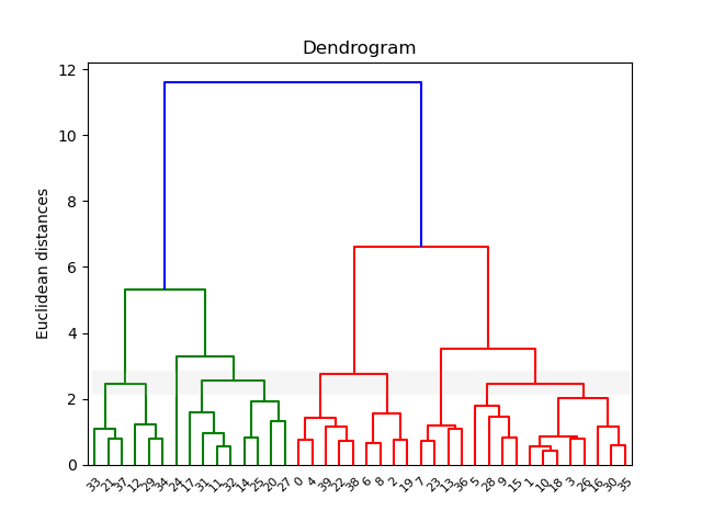
The single line that passes with more dendrograms is considered to be the optimal number of clusters. For this example, I have put a grey line to indicate that have the line passed the most dendrograms.
Alright, we have our optimal number of clusters = 4 now it's time to build our model.
#Fitting Hierarchical Clustering to the dataset
from sklearn.cluster import AgglomerativeClustering
hc_model = AgglomerativeClustering(n_clusters = 4, affinity = 'euclidean', linkage = 'ward')
Here we have used the agglomerative ‘bottom up’ approach with euclidean distance and with the ‘Ward’ Linkage method to seed the centroids.
Ward’s is said to be the most suitable method for quantitative variables.
Time to predict
#Predicting with new data
y_hc = hc_model.fit_predict(X_train)
y_hc1 = hc_model.fit_predict(X_test)
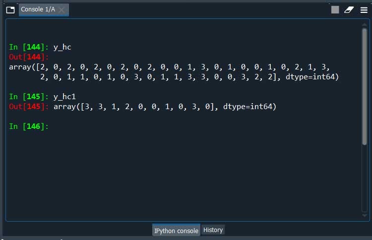
Here we are we have our clusters.
Let me put all of the pieces together.
#H_Clustering
#Importing the libraries
import numpy as np
import matplotlib.pyplot as plt
import pandas as pd
#Importing the dataset
dataset = pd.read_csv('crime_data.csv')
#drop the missing values
dataset = dataset.dropna()
X = dataset.iloc[:,2:].values
#Normalization
from sklearn.preprocessing import StandardScaler
sc_X = StandardScaler()
X=sc_X.fit_transform(X)
#Splitting the dataset into the Training set and Test set
#Here we dont have a dependent variable becoz its an unsupervised #learning so its not required However we will split the data to test #our model with new data
from sklearn.model_selection import train_test_split
X_train, X_test = train_test_split(X, test_size = 0.2, random_state = 0)
#Using the dendrogram to find the optimal number of clusters
import scipy.cluster.hierarchy as sch
dendrogram = sch.dendrogram(sch.linkage(X_train, method = 'ward'))
plt.title('Dendrogram')
plt.xlabel('Customers')
plt.ylabel('Euclidean distances')
plt.show()
#Fitting Hierarchical Clustering to the dataset
from sklearn.cluster import AgglomerativeClustering
hc_model = AgglomerativeClustering(n_clusters = 4, affinity = 'euclidean', linkage = 'ward')
#Predicting with new data
y_hc = hc_model.fit_predict(X_train)
y_hc1 = hc_model.fit_predict(X_test)
Ya! Probably you already have used the above 2 methods more than I do. Now try to move to something new. Density-Based Spatial (DBSCAN ) Clustering.

Density-Based Spatial (DBSCAN ) Clustering.
DBSCAN is a clustering method that is used in machine learning to separate clusters of high density from clusters of low density.
It does a great job of finding clusters in the data that have a high density of observations, versus areas of the data that are not very dense with observations.
DBSCAN divides the dataset into n dimensions. For each point in the dataset DBSCAN forms an’ N’ dimensional shape around the data point and then counts how many data points fall within that shape. Then it counts the shapes as a cluster. This repeats iteratively by going through each individual point within the cluster and counting the number of other data points nearby.
The only disadvantage of DBSCAN is it doesn’t work well when dealing with clustering of varying densities also it struggles to cluster data of similar density.
DBSCAN has 4 important parts/components.
1.) Epcilan 2.) Min pts 3.) Core Point 4.) Border Points 5.) Noise Point
1.) Core Point: a point is a core if it has more than Min Pts points within eps.
2.) Min Pts: Minimum number of neighbors(data points) within eps radius larges the data the layer value of Min Pts must be chosen. As a general rule, the minimum MinPts can be derived from the number of dimension D in the dataset as MinPts >=D+1
The Minimum value of Min Pts must be chosen at least 3
3.) Border Point: a point which has fewer than Min Pts within eps buy it is in the neighborhood of a core point.
4.) Noise basically like an Outlier: a point that is not a core point or border point.
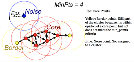
Suppose it doesn’t satisfy the min.pts but we have at least one core point inside of the boundary. Then it becomes a border point.
Let’s see how can we apply DBSCAN using python.
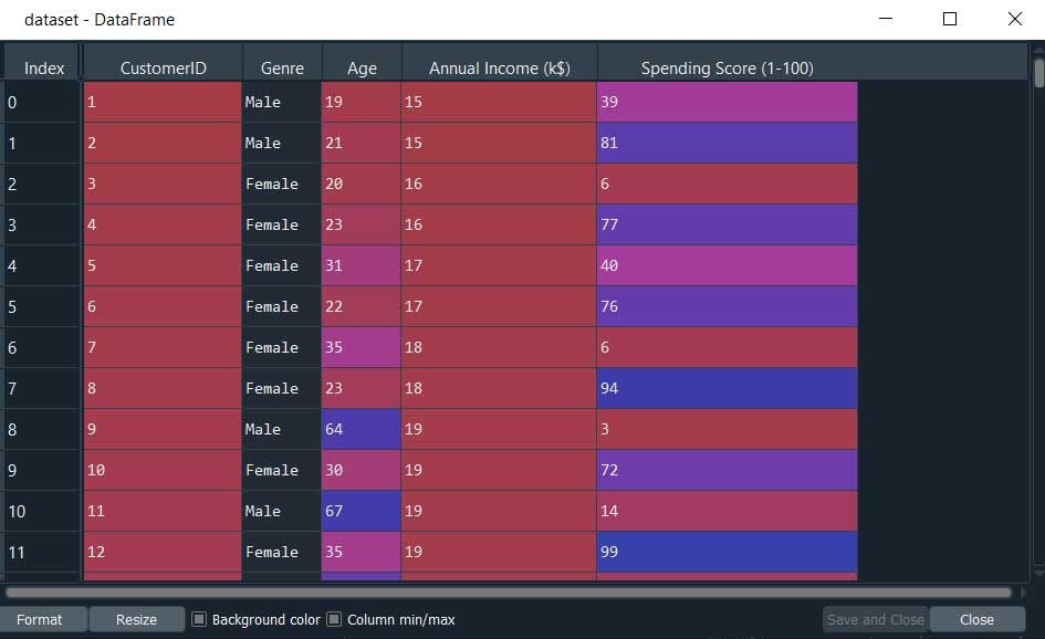
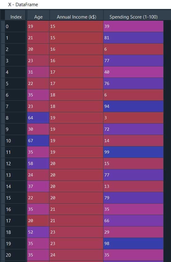
Here are our dataset looks like
import numpy as np
from sklearn.cluster import DBSCAN
from sklearn import metrics
from sklearn.datasets.samples_generator import make_blobs
from sklearn import datasets
import pandas as pd
import matplotlib as plt
#Importing the dataset
dataset = pd.read_csv('Mall_Customers.csv')
X = dataset.iloc[:, [3, 4]].values
#feature scaling/Normalization
from sklearn.preprocessing import StandardScaler
sc = StandardScaler()
X = sc.fit_transform(X)
#apply model
db = DBSCAN(eps=0.3, min_samples=10).fit(X)
'''where min_samples is
The number of samples (or total weight) in a neighborhood for a point to be considered as a core point. This includes the point itself.'''
#eps = The maximum distance between two samples for one to be considered as in the neighborhood of the other.
#create a dummy columns
core_samples_mask = np.zeros_like(db.labels_, dtype=bool)
#uses index values of db if True keep True else False
core_samples_mask[db.core_sample_indices_] = True
labels = db.labels_
#ELSE if we want only the outliers
#counter gives count of each unique values
from collections import Counter
print(Counter(db.labels_))
print(X[db.labels_==-1])
#Number of clusters in labels, ignoring noise if present.
n_clusters_ = len(set(labels)) - (1 if -1 in labels else 0)
print(labels)
#Plot result
import matplotlib.pyplot as plt
#Black removed and is used for noise instead.
unique_labels = set(labels)
colors = ['y', 'b', 'g', 'r']
print(colors)
for k, col in zip(unique_labels, colors):
if k == -1:
#Black used for noise.
col = 'k'class_member_mask = (labels == k)
xy = X[class_member_mask & core_samples_mask]
plt.plot(xy[:, 0], xy[:, 1], 'o', markerfacecolor=col,
markeredgecolor='k',
markersize=6)
xy = X[class_member_mask & ~core_samples_mask]
plt.plot(xy[:, 0], xy[:, 1], 'o', markerfacecolor=col,
markeredgecolor='k',
markersize=6)
plt.title('number of clusters: %d' %n_clusters_)
plt.show()
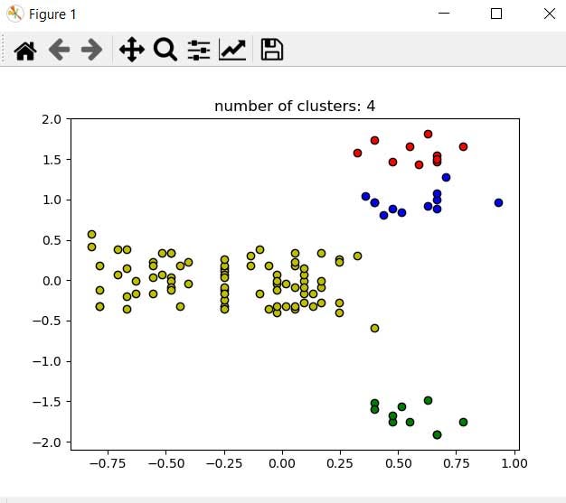
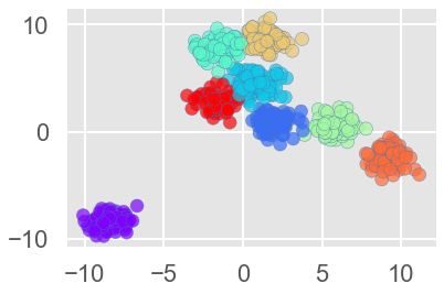
Here we have our data clustered from the density of data points.
Next, let’s understand the Hierarchical version of DBSCAN
HDBSCAN — a Hierarchical Density-Based Spatial Clustering
Why do K-means fail? K-means performs poorly because the underlying assumptions on the clusters are not met. It is parametric algorithms parameterized by the K cluster centroids the centers of Gaussian spheres K-means performs best when clusters are
Ø Round or spherical, Equally sized, Equally dense
Ø Most dense in the center of the sphere
Ø Most contaminated by noise/outliers
HDBSCAN uses a density-based approach which makes few implicit assumptions about the clusters. It is a non-parametric method that looks for a cluster hierarchy shaped by the multi-variate modes of the underlying distribution. Rather than looking for clusters with a particular shape. It looks for regions of the data that are denser than the surrounding space.
Cluster.condensed_tree_.plot()
This particular plot may be useful for assessing the quality of your clusters and can help with fine-tuning the hyper-parameters.
The 2 main parameters of HDBSCAN are min_samples & mincluster size
Here we try to estimate this using the core distances which is the distance to the K-nearest neighbor. The hyperparameter K here is referred to as min_samples
The simple intuition for min_samples does is to provide a measure of how conservative you want your clustering to be. The larger the value of min_samples you provide the more conservatives the clustering — more points will be declared as noise and clusters will be restricted to progressively more dense areas.
Regular DBSCAN is amazing at clustering data of varying shapes but falls short of clustering data of varying density.
#HDBSCAN
import numpy as np
import matplotlib.pyplot as plt
import seaborn as sns
import sklearn.datasets as data
%matplotlib inline
sns.set_context('poster')
sns.set_style('white')
sns.set_color_codes()
plot_kwds = {'alpha' : 0.5, 's' : 80, 'linewidths':0}
''' sklearn has facilities for generating sample clustering data '''
moons, _ = data.make_moons(n_samples=50, noise=0.05)
blobs, _ = data.make_blobs(n_samples=50, centers=[(-0.75,2.25), (1.0, 2.0)], cluster_std=0.25)
test_data = np.vstack([moons, blobs])
plt.scatter(test_data.T[0], test_data.T[1], color='b', **plot_kwds)
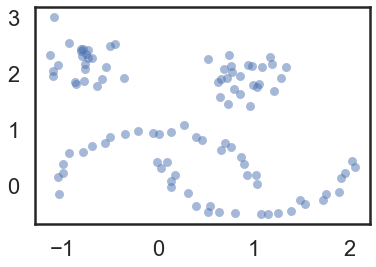
Our sample dataset (test_data)
import hdbscan
clusterer = hdbscan.HDBSCAN(min_cluster_size=5, gen_min_span_tree=True)
clusterer.fit(test_data)
Here we are to apply hdbscan we will call the hdbscan function.
####optional########################################
model=clusterer.fit(test_data)
#cluster values
labels=model.labels_
from collections import Counter
print(Counter(model.labels_))
#outliers/noise
label_testdata = test_data[model.labels_==-1]
The parameters of HDBSCAN
HDBSCAN(algorithm=’best’, alpha=1.0, approx_min_span_tree=True,
gen_min_span_tree=True, leaf_size=40, memory=Memory(cachedir=None),
metric=’euclidean’, min_cluster_size=5, min_samples=None, p=None)
Now we have clustered our data based on HDBSCAN. But how can we interpret to use them?
1st Transform the space/data according to the density/sparsity which we already did.
2nd Build the minimum spanning tree of the distance weighted graph.
3rd Construct a cluster hierarchy of connected components.
4th Condense the cluster hierarchy based on minimum cluster size.
Finally extract the stable clusters from the condensed tree.
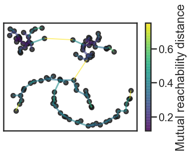
Now let's build the minimum spanning tree
#We can build the minimum spanning tree via Prim’s algorithm
clusterer.minimum_spanning_tree_.plot(edge_cmap=’viridis’,
edge_alpha=0.6,
node_size=80,
edge_linewidth=2)
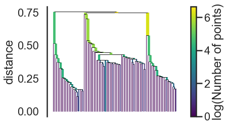
3. Now we can construct a cluster hierarchy
#Build the cluster hierarchy
clusterer.single_linkage_tree_.plot(cmap=’viridis’, colorbar=True)
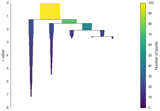
4. Condense the cluster hierarchy based on minimum cluster size.
This is the first step of cluster extraction is condensing down the large and complicated cluster hierarchy into a smaller tree.
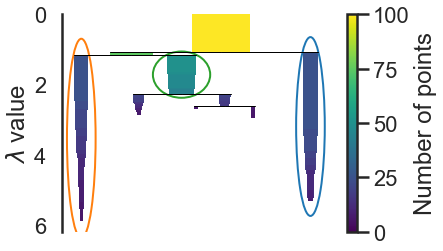
clusterer.condensed_tree_.plot()
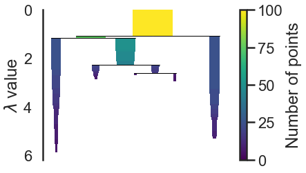
We can now see the hierarchy as a dendrogram, the width (and color) of each branch representing the number of points in the cluster at that level.
#we want the clusters that persist and have a longer lifetime, short clusters are probably merely artifacts of the single linkage approach. If we wish to know the clusters/branches selected by the HDBSCAN* algorithm we can pass select_clusters=True
clusterer.condensed_tree_.plot(select_clusters=True, selection_palette=sns.color_palette())
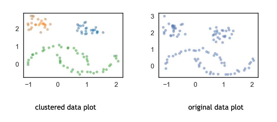
Comparison Clustered Data vs Non-Clustered Data
#clustered dataset plot
palette = sns.color_palette()
cluster_colors = [sns.desaturate(palette[col], sat)
                  if col >= 0 else (0.5, 0.5, 0.5) for col, sat in
                  zip(clusterer.labels_, clusterer.probabilities_)]
plt.scatter(test_data.T[0], test_data.T[1], c=cluster_colors, **plot_kwds)
#original dataset plot
plt.scatter(test_data.T[0], test_data.T[1], color='b', **plot_kwds)
Next, we have Mini — Batch size clustering approach

Mini — Batch size clustering approach.
K-means is one of the most popular clustering algorithms, mainly because of this speed. But with the increasing size of the dataset which needs to be analyzed, the computation time of K-means increases because it needs the whole dataset to be loaded in the main memory. This effects the performance and its computationally costly. To overcome this situation Mini Batch K-means clustering algorithm was introduced.
Mini-Batch K-means works similarly to the K-means algorithm however it uses small random batches of data of a fixed size, so they can be stored in memory. Thus it has a huge impact on speed as computational cost.
Let’s see how can we perform Mini-Batch Clustering
#mini-batch size Clustering
#Load libraries
from sklearn import datasets
from sklearn.preprocessing import StandardScaler
from sklearn.cluster import MiniBatchKMeans
from sklearn.cluster import KMeans
import matplotlib.pyplot as plt
import pandas as pd
#Load data
iris = datasets.load_iris()
X = iris.data
#convert to dataframe
X=pd.DataFrame(X)
#Standarize features
scaler = StandardScaler()
X_std = scaler.fit_transform(X)
#Create k-mean object
clustering = MiniBatchKMeans(n_clusters=3, random_state=0, batch_size=100)
#OR
#perform the mini batch K-means
clustering = MiniBatchKMeans(init ='k-means++', n_clusters = 4,
batch_size = 100, n_init = 10,
max_no_improvement = 10, verbose = 0)
#N_int=10 refers maximum number of iterations. No. of times the K-means algorithm will be run with different centroid seeds.
#Max_non_improvement: 10 refers control early stopping based on the consecutive number of mini batches that dosnt yield an improvement on the smoothen inertia.
#To disable convergence detection based on intertia. Set max_no_improvement to None.
#Train model
model = clustering.fit(X_std)
#to get the number of clusters
model.n_clusters
#to get the labels
labels=model.labels_
#counter gives count of each unique values
from collections import Counter
print(Counter(model.labels_))
That’s it easy, isn’t it!
Next, Let’s move on with another interesting type of clustering called ‘Fuzzy Clustering’.
Fuzzy Clustering
Fuzzy clustering is a clustering method where data points can belong to more than one group(‘cluster’)
There are 2 ways of clustering we might not know,,
One is ‘Hard Clustering’ and the other was is ‘Soft Clustering / Fuzzy Clustering’
In ‘hard clustering’ each data point can only be 1 cluster but in ‘soft clustering’ or ‘fuzzy clustering’ data point can belong to more than one group.
Fuzzy clustering uses least squares to find the optimal location for any data point. This optimal location may be in a probability space between two (or more) clusters.
Fuzzy clustering algorithms (FCM) are again divided into 2 areas
1.) Classical fuzzy clustering and 2.) Shape-based fuzzy
1.) Classical Fuzzy Clustering
a.) Fuzzy C-Means algorithm (FCM). is widely used algorithm is practically identical to the K-means algorithm. A data point can theoretically belong to one or all groups. Subtype includes Possibilistic C-Means(PCM), Fuzzy Possibilistic C-Means (FPCM), and Possibilistic Fuzzy C-Means (PFCM).
2.) Shape-based fuzzy clustering
a.) Circular shaped: circular-shaped (CS) algorithms are what constraints data point to a circular shape. When this algorithm is incorporated into Fuzzy C-Means it’s called CS-FCM
b.) Elliptical Shaped: an algorithm that constrains points to elliptical shapes. Used in the GK algorithm.
c.) Generic shaped. More real-life objects are neither circular nor elliptical, the generic algorithm allows for clusters of any shape.
Well as of now we will concentrate more with the simple Fuzzy C-Means Clustering.
Steps to perform fuzzy algorithm:
Step 1: Initialize the data points into the desired number of clusters randomly.
Step 2: Find out the centroids
Step 3: Find out the distance of each point from the centroid
Step 4: Updating membership values
Step 5: Repeat steps(2–4) until the constant values are obtained for the membership.
Let’s see how we can perform the fuzzy clustering.
import numpy as np, numpy.random
import pandas as pd
from scipy.spatial import distance
k =3
p = 2
from sklearn import datasets
from sklearn.preprocessing import StandardScaler
import pandas as pd
#Load data
iris = datasets.load_iris()
X = iris.data
#Standarize features
scaler = StandardScaler()
X1 = scaler.fit_transform(X)
#convert to dataframe
X1 = pd.DataFrame(X1)
X=X1
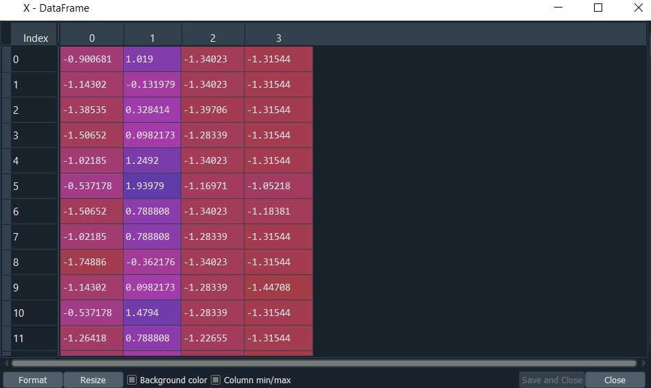
X = pd.DataFrame(X)
This is our dataset.
#Print the number of data and dimension
n = len(X)
d = len(X.columns)
addZeros = np.zeros((n, 1))
X = np.append(X, addZeros, axis=1)
print("The FCM algorithm: \n")
print("The training data: \n", X)
print("\nTotal number of data: ",n)
print("Total number of features: ",d)
print("Total number of Clusters: ",k)
#Create an empty array of centers
C = np.zeros((k,d+1))
#print(C)
#Randomly initialize the weight matrix
weight = np.random.dirichlet(np.ones(k),size=n)
print("\nThe initial weight: \n", np.round(weight,2))
for it in range(3): # Total number of iterations
#Compute centroid
for j in range(k):
denoSum = sum(np.power(weight[:,j],2))
sumMM =0
for i in range(n):
mm = np.multiply(np.power(weight[i,j],p),X[i,:])
sumMM +=mm
cc = sumMM/denoSum
C[j] = np.reshape(cc,d+1)
#print("\nUpdating the fuzzy pseudo partition")
for i in range(n):
denoSumNext = 0for j in range(k):
denoSumNext += np.power(1/distance.euclidean(C[j,0:d], X[i,0:d]),1/(p-1))
for j in range(k):
w = np.power((1/distance.euclidean(C[j,0:d], X[i,0:d])),1/(p-1))/denoSumNext
weight[i,j] = w
print("\nThe final weights: \n", np.round(weight,2))
It's Time to find out our fuzzy clusters.
for i in range(n):
cNumber = np.where(weight[i] == np.amax(weight[i]))
X[i,d] = cNumber[0]
print("\nThe data with cluster number: \n", X)
This is will display the data along with the cluster number else simply click X from variable explorer.
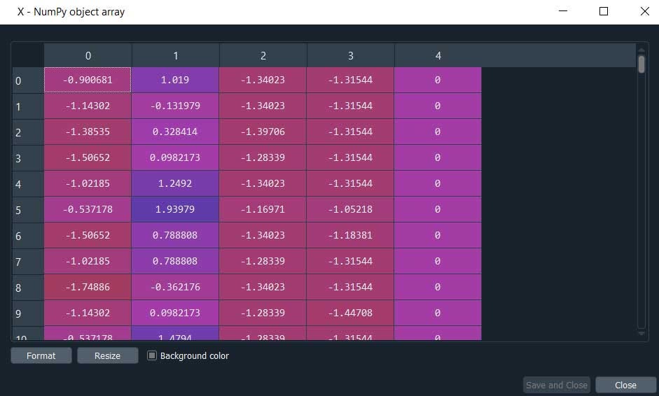
Here we are, the column ‘4’ has the cluster values.
Let me put all the pieces together so you can use them as a template.
#Fuzzy c means clustering algorithm
import numpy as np, numpy.random
import pandas as pd
from scipy.spatial import distance
k =3
p = 2
from sklearn import datasets
from sklearn.preprocessing import StandardScaler
import pandas as pd
# Load data
iris = datasets.load_iris()
X = iris.data
# Standarize features
scaler = StandardScaler()
X1 = scaler.fit_transform(X)
#convert to dataframe
X1 = pd.DataFrame(X1)
X=X1
X = pd.DataFrame(X)
#-------------------------------------------------------
#Print the number of data and dimension
n = len(X)
d = len(X.columns)
addZeros = np.zeros((n, 1))
X = np.append(X, addZeros, axis=1)
print("The FCM algorithm: \n")
print("The training data: \n", X)
print("\nTotal number of data: ",n)
print("Total number of features: ",d)
print("Total number of Clusters: ",k)
#Create an empty array of centers
C = np.zeros((k,d+1))
#print(C)
#Randomly initialize the weight matrix
weight = np.random.dirichlet(np.ones(k),size=n)
print("\nThe initial weight: \n", np.round(weight,2))
for it in range(3): # Total number of iterations
# Compute centroid
for j in range(k):
denoSum = sum(np.power(weight[:,j],2))
sumMM =0
for i in range(n):
mm = np.multiply(np.power(weight[i,j],p),X[i,:])
sumMM +=mm
cc = sumMM/denoSum
C[j] = np.reshape(cc,d+1)
#print("\nUpdating the fuzzy pseudo partition")
for i in range(n):
denoSumNext = 0
for j in range(k):
denoSumNext += np.power(1/distance.euclidean(C[j,0:d], X[i,0:d]),1/(p-1))
for j in range(k):
w = np.power((1/distance.euclidean(C[j,0:d], X[i,0:d])),1/(p-1))/denoSumNext
weight[i,j] = w
print("\nThe final weights: \n", np.round(weight,2))
for i in range(n):
cNumber = np.where(weight[i] == np.amax(weight[i]))
X[i,d] = cNumber[0]
print("\nThe data with cluster number: \n", X)
#Sum squared error calculation
SSE = 0
for j in range(k):
    for i in range(n):
        SSE += np.power(weight[i,j],p)*distance.euclidean(C[j,0:d], X[i,0:d])
print("\nSSE: ",np.round(SSE,4))
Now the some of the widely used applications of Fuzzy Clustering are
Bio-informatics:
One way to use it for pattern recognition technique to analyze gene expression data from microarrays or others. In this case, genes with similar expression/patterns are grouped into the same clusters. Because fuzzy clustering allows genes to belong to more than one cluster. It allows for the identification of genes that are conditionally co-regulated.
Marketing: customers can be grouped into fuzzy clusters based on their needs, brand choices, psycho-graphic profiles, or other marketing-related partitions.
Further, it is used for image analysis, medicine, psychology, economics, and many other disciplines.
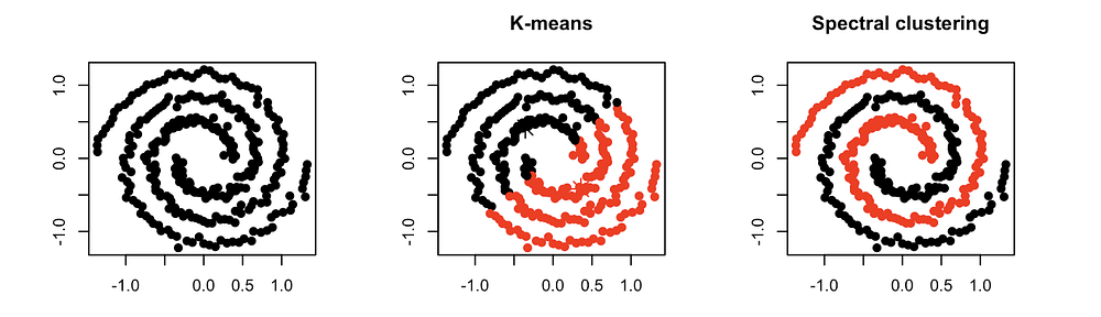
Next another interesting Clustering technique we have is called ‘Spectral Clustering’

Spectral Clustering
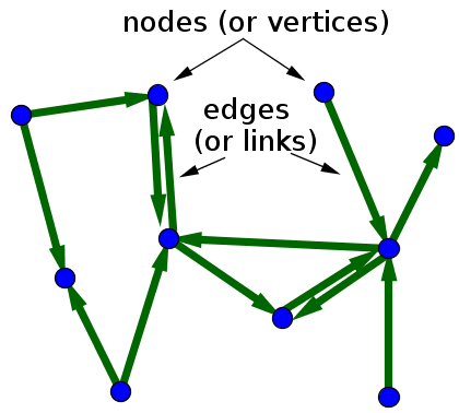
Spectral clustering is a growing clustering algorithm that also outperforms traditional clustering algorithm in many cases. It treats each data point as a graph node and thus transforms the clustering problem into a graph-partitioning problem.
Spectral clustering basically consists of 3 steps:
- Building the Similarity Graph: this step builds the Similarity Graph in the form of an adjacency matrix which is represented by A. The adjacency matrix can be built in the following manner:
- Epsilon-neighborhood Graph. A parameter epsilon is fixed beforehand. Then each point is connected to all the points which lie in its epsilon-radius. If all the distances between any two points are similar in scale then typically they do not provide any additional information. This, in this case, the graph build is an undirected and unweighted graph.
- K-Nearest Neighbors. A parameter K is fixed beforehand. Then for two vertices u and v, an edge is directed from u to v only if v is among the K-nearest neighbors of u. Note that this leads to the formation of a weighted and directed graph because it is not always the case that for each u having u as one of the k-nearest neighbors, it will be the same case for v having u among its K-nearest neighbors.
To make this graph undirected, one of the following approaches are followed:
1. Direct an edge from u to v and from v to u if either v is among the k-nearest neighbors of u OR u is among the k-nearest neighbors of v.
2. Direct an edge from u to v and from v to u if v is among the k-nearest neighbors of u AND u is among the k-nearest neighbors of v.
- Fully-Connected Graph: To build this graph, each point is connected with an undirected edge-weighted by the distance between the two points to every other point. Since this approach is used to model the local neighborhood relationships thus typically the Gaussian similarity metric is used to calculate the distance.
2. Projecting the data onto a lower Dimensional Space: This step is done to account for the possibility that members of the same cluster may be far away in the given dimensional space. Thus the dimensional space is reduced so that those points are closer in the reduced dimensional space and thus can be clustered together by a traditional clustering algorithm. It is done by computing the Graph Laplacian Matrix
3. Clustering the Data: This process mainly involves clustering the reduced data by using any traditional clustering technique — typically K-Means Clustering.
Alright Now, let's understand this with the help of an example.
First, we will load all the libraries and some data pre-processing.
#Spectral Clustering
import pandas as pd
import matplotlib.pyplot as plt
from sklearn.cluster import SpectralClustering
from sklearn.preprocessing import StandardScaler, normalize
from sklearn.decomposition import PCA
from sklearn.metrics import silhouette_score
#Loading the data
X = pd.read_csv('creditcard.csv')
#Dropping the CUST_ID column from the data
X = X.drop('CUST_ID', axis = 1)
#Handling the missing values if any
X.fillna(method ='ffill', inplace = True)
X.head()
#Preprocessing the data to make it visualizable
#Scaling the Data
scaler = StandardScaler()
X_scaled = scaler.fit_transform(X)
#Normalizing the Data
X_normalized = normalize(X_scaled)
#Converting the numpy array into a pandas DataFrame
X_normalized = pd.DataFrame(X_normalized)
# Reducing the dimensions of the data
pca = PCA(n_components = 2)X_principal = pca.fit_transform(X_normalized)
X_principal = pd.DataFrame(X_principal)
X_principal.columns = ['P1', 'P2']
X_principal.head()
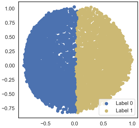
Now we can perform Spectral Clustering using 2 different ways
One with radial basis function ‘rbf’ and another ‘K-nearest neighbors’
#two different Spectral Clustering models with different values for the parameter ‘affinity’
#a) affinity = ‘rbf’
#Building the clustering model
spectral_model_rbf = SpectralClustering(n_clusters = 2, affinity ='rbf')
#Training the model and Storing the predicted cluster labels
labels_rbf = spectral_model_rbf.fit_predict(X_principal)
#Building the label to colour mapping
colours = {}
colours[0] = 'b'
colours[1] = 'y'
#Building the colour vector for each data point
cvec = [colours[label] for label in labels_rbf]
#Plotting the clustered scatter plot
b = plt.scatter(X_principal['P1'], X_principal['P2'], color ='b');
y = plt.scatter(X_principal['P1'], X_principal['P2'], color ='y');
plt.figure(figsize =(9, 9))
plt.scatter(X_principal['P1'], X_principal['P2'], c = cvec)
plt.legend((b, y), ('Label 0', 'Label 1'))
plt.show()
#b) affinity = ‘nearest_neighbors’
#Building the clustering model
spectral_model_nn = SpectralClustering(n_clusters = 2, affinity ='nearest_neighbors')
#Training the model and Storing the predicted cluster labels
labels_nn = spectral_model_nn.fit_predict(X_principal)
Now we can evaluate which affinity parameter is performing well.
#Step 5: Evaluating the performances
#List of different values of affinity
affinity = ['rbf', 'nearest-neighbours']
#List of Silhouette Scores
s_scores = []
#Evaluating the performance
s_scores.append(silhouette_score(X, labels_rbf))
s_scores.append(silhouette_score(X, labels_nn))
print(s_scores)
#Plotting a Bar Graph to compare the models
plt.bar(affinity, s_scores)
plt.xlabel('Affinity')
plt.ylabel('Silhouette Score')
plt.title('Comparison of different Clustering Models')
plt.show()
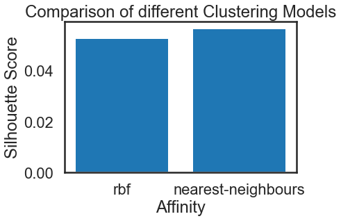
Alright, the ‘nearest-neighbors’ is performing better than ‘rbf’ in our Spectral clustering.
This is how we can perform Spectral Clustering. I hope you are able to capture the intuition of how and when to apply Spectral Clustering in the shortest and the simplest way.
Next, we have another Powerful Clustering method call MeanShift Clustering
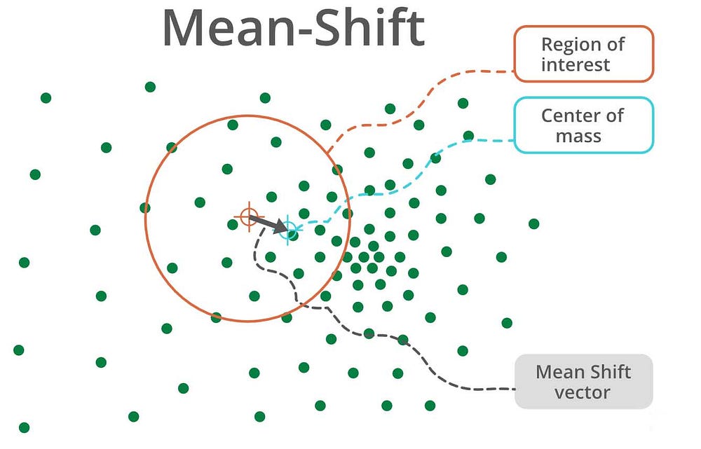
Mean-Shift Clustering
Meanshift is another powerful clustering algorithm used in unsupervised learning. Unlike K-means clustering, it does not make any assumptions; hence it is a non-parametric algorithm.
It assigns the data points to the clusters iteratively by shifting points towards the mode( highest density of data points in the region)
The difference between K-means algorithm and Mean-Shift is that Mean Shift doesn’t need to specify the number of clusters in advance because the number of clusters will decide by the algorithm.
Working of Mean-Shift:
- Step 1 − First, start with the data points assigned to a cluster of their own.
- Step 2 − Next, this algorithm will compute the centroids.
- Step 3 − In this step, the location of new centroids will be updated.
- Step 4 − Now, the process will be iterated and moved to the higher density region.
- Step 5 − At last, it will be stopped once the centroids reach a position from where it cannot move further.
I have collected a few of its advantages and disadvantages from various sources as well as its applications.
Here it is.
Advantages of Mean-Shift
· It does not need to make any model assumption as in K-means or Gaussian mixture.
· It can also model the complex clusters which have nonconvex shape.
· It only needs one parameter named bandwidth which automatically determines the number of clusters.
· There is no issue of local minima as in K-means.
· No problem generated from outliers.
Disadvantages:
· Mean-shift algorithm does not work well in case of high dimension, where a number of clusters change abruptly.
· We do not have any direct control over the number of clusters but in some applications, we need a specific number of clusters.
· It cannot differentiate between meaningful and meaningless modes.
Applications:
As far as my experience Mean-shift can be used for visual tracking and in the field of image processing and computer vision.
Now let’s see how can we perform Mean-shift Clustering.
For this example we will use the preloaded iris dataset then we will perform our regular data pre-processing steps like Scaling.
import numpy as np, numpy.random
import pandas as pd
import matplotlib.pyplot as plt
from scipy.spatial import distance
from sklearn import datasets
from sklearn.preprocessing import StandardScaler
#Load data
iris = datasets.load_iris()
X = iris.data
#Standarize features
scaler = StandardScaler()
X = scaler.fit_transform(X)
We will use sklearn.cluster to import MeanShift
from sklearn.cluster import MeanShift
ms = MeanShift()
ms.fit(X)
labels = ms.labels_
cluster_centers = ms.cluster_centers_
print(cluster_centers)
#number of clusters
n_clusters_ = len(np.unique(labels))
print("Estimated clusters:", n_clusters_)
colors = 10*['r.','g.','b.','c.','k.','y.','m.']
for i in range(len(X)):
plt.plot(X[i][0], X[i][1], colors[labels[i]], markersize = 3)
plt.scatter(cluster_centers[:,0],cluster_centers[:,1],
marker = ".",color = 'k', s = 20, linewidths = 5, zorder = 10)
plt.show()
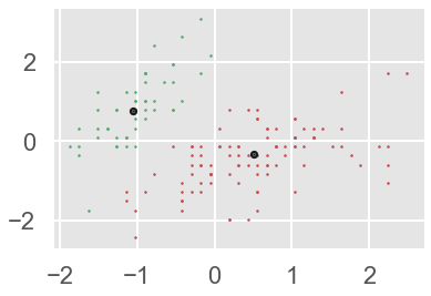
Here we are. We have two Mean-Shift clusters.
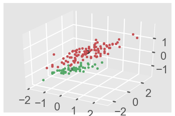
We can also use the Axes3D function to plot this in 3D format.
#3D plot-------
from mpl_toolkits.mplot3d import Axes3D
colors = 10*['r','g','b','c','k','y','m']
fig = plt.figure()
ax = fig.add_subplot(111,projection ='3d')
for i in range(len(X)):
ax.scatter(X[i][0], X[i][1],X[i][2], c = colors[labels[i]], marker='o')
ax.scatter(cluster_centers[:,0],cluster_centers[:,1],cluster_centers[:,2],
marker = ".",color = 'k', s = 20, linewidths = 5, zorder = 10)
plt.show()
plt.draw()
Alright, next we have a powerful Clustering technique specially designed and optimized for big data called BIRCH Clustering.
Balanced Iterative Reducing and Clustering using Hierarchies (BIRCH)
Clustering algorithms like K-means clustering do not perform clustering very efficiently when it comes to processing large datasets with a limited amount of resources that is system memory or a slower CPU. This is where Balanced Iterative Reducing and Clustering using Hierarchies (BIRCH) comes in.
BIRCH is an unsupervised clustering algorithm that is used to cluster big data by first generating a small and compact summary of the large dataset that retains as much information as possible. Then this smaller summary is clustered instead of clustering the larger dataset.
BIRCH has one major disadvantage is it can only process numeric values and no categorical attributes should be present.
There are 2 important terms of BIRCH:
Clustering Feature(CF) and CF-Tree.
Clustering Feature (CF)
BIRCH summarizes large datasets into smaller, dense regions called Clustering Feature(CF) entries. Formally, a Clustering Feature entry is defined as an ordered triple (N,LS,SS) where ’N’ is the number of data points in the cluster, ‘LS’ is the linear sum of the data points and ‘ss’ is the squared sum of the data points in the cluster. It is possible for a CF entry to be composed of other CF entries.
CF-Tree:
The CF Tree is the actual compact representation that we have been speaking of so far. A CF tree where each leaf node contains a sub-cluster. Every entry in a CF tree contains a pointer to a child node and a CF entry made up of the sum of CF entries in the child nodes. There is a maximum number of entries in each leaf node. This maximum number is called the threshold.
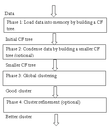
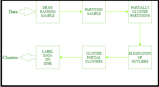
Stages of BIRCH algorithm
> Phase 1: Load data into memory
- Scan DB and load data into memory by building a CF tree. If memory is exhausted rebuild the tree from the leaf node.
> Phase 2: Condense data
- Resize the data set by building a smaller CF tree.
- Remove more outliers
- Condensing is optional
> Phase 3: Global clustering
- Use existing clustering algorithm (example K-means, HC) on CF entries
> Phase 4: Cluster refining (optional)
- Fixes the problem with CF trees where the same valued data points may be assigned to different lead entries.
A few of the widely used applications of BIRCH are Pixel classification in images, image compression and off course with very large data sets.
Now let’s see how can we perform BIRCH with the help of an example.
However, will developing the BIRCH we need to take care of 3 important parameters
threshold: the threshold is the maximum number of data points a sub-cluster in the leaf node of the CF tree can hold.
branching_factor: This parameter specifies the maximum number of CF sub-clusters in each node (internal node).
n_clusters: The number of clusters to be returned after the entire BIRCH algorithm is complete i.e., number of clusters after the final clustering step. If set to None, the final clustering step is not performed and intermediate clusters are returned.
#Birch Clustering
#Import required libraries and modules
import matplotlib.pyplot as plt
from sklearn.datasets.samples_generator import make_blobs
from sklearn.cluster import Birch
#Code: To create 8 clusters with 600 randomly generated samples and then plotting the results in a scatter plot.
#Generating 600 samples using make_blobs
dataset, clusters = make_blobs(n_samples = 600, centers = 8, cluster_std = 0.75, random_state = 0)
#Creating the BIRCH clustering model
model = Birch(branching_factor = 50, n_clusters = None, threshold = 1.5)
'''
threshold :  threshold is the maximum number of data points a sub-cluster in the leaf node of the CF tree can hold.
branching_factor : This parameter specifies the maximum number of CF sub-clusters in each node (internal node).
n_clusters : The number of clusters to be returned after the entire BIRCH algorithm is complete i.e., number of clusters after the final clustering step. If set to None, the final clustering step is not performed and intermediate clusters are returned.
'''
#Fit the data (Training)
model.fit(dataset)
#Predict the same data
pred = model.predict(dataset)
#Creating a scatter plot
plt.scatter(dataset[:, 0], dataset[:, 1], c = pred, cmap = 'rainbow', alpha = 0.7, edgecolors = 'b')
plt.show()
cluster_labels=model.labels_
import numpy as np
np.unique(cluster_labels)
#output
#Out[125]: array([0, 1, 2, 3, 4, 5, 6, 7])
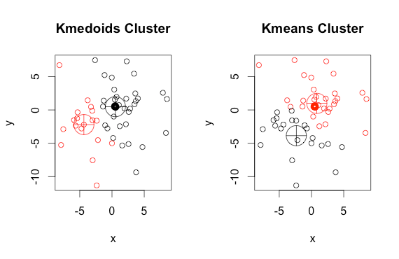
Next, we have Clustering based on Partitioning Around Medoids (k-Medoids)
K-Medoids
K-Medoids is also known as the Partitioning Around Medoids algorithm was proposed in 1987 by Kaufman and Rousseeuw
Both the k -means and k -medoids algorithms are partitional (breaking the dataset up into groups). K-means attempts to minimize the total squared error, while k-medoids minimize the sum of dissimilarities between points labeled to be in a cluster and a point designated as the center of that cluster(medoid)
K-Medoid Steps include:
1.) Select K random points out of the n data points as the medoids
2.) Calculate the Cost: the dissimilarity of each non-medoid point with the medoids is calculated and tabulated.
3.) Randomly select one non-medoid point and recalculate the cost.
In other words, while the cost decreases:
For each medoid m, for each data o point which is not a medoid:
Swap m and o, associate each data point to the closest medoid, recompute the cost. If the total cost is more than that in the previous step, undo the swap.
Advantages:
1. It is simple to understand and easy to implement.
2. K-Medoid algorithm is fast and converges in a fixed number of steps.
Also, it is more robust to noise and outliers as compared to k-means as it minimizes a sum of pairwise dissimilarities instead of a sum of Squared Euclidean Distances.
However, the disadvantage is that is not suitable for clustering non-spherical (arbitrary shaped) groups of data. This is because it depends on minimizing the distances between the non-medoid objects and the medoid(cluster center)
#KMedoids
#pip install scikit-learn extra
from sklearn_extra.cluster import KMedoids
import numpy as np
#from the file import KMedoids
X = np.asarray([[1, 2], [1, 4], [1, 0],[4, 2], [4, 4], [4, 0]])
kmedoids = KMedoids(n_clusters=2, random_state=0).fit(X)
kmedoids.labels_
kmedoids.predict([[0,0], [4,4]])
kmedoids.cluster_centers_
kmedoids.inertia_
Moving on to the next Method is Ordering Points To Identify The Clustering Structure (OPTICS)

OPTICS Clustering
Ordering Points To Identify Cluster Structure (OPTICS) ) is a density-based clustering technique that allows partitioning data into groups with similar characteristics(clusters)
Its addresses one of the DBSCAN’s major weaknesses. The problem of detecting meaningful clusters in data of varying density.
In density-based clustering, clusters are defined as dense regions of data points separated by low-density regions.
It adds two more terms to the concepts of DBSCAN clustering. They are:
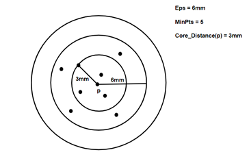
- Core Distance: it is the minimum value of radius required to classify a given point as a core point. if the given point is not a Core point, then its Core Distance is undefined.
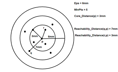
2. Reachability Distance: it is defined with respect to another data point ‘q’. The Reachability distance between a point p and q . Note that The Reachability Distance is not defined if ‘q’ is not a Core point.
Few advantages:
· OPTICS clustering doesn’t require a predefined number of clusters in advance.
· Clusters can be of any shape, including non-spherical ones.
· Able to identify outliers(noise data)
Disadvantages:
· It fails if there are no density drops between clusters.
· It is also sensitive to parameters that define density( radius and the minimum number of points) and proper parameter settings require domain knowledge.
Now let’s understand the coding part.
First, we will load our dataset and perform a few data pre-processing steps like scaling.
#OPTICS Clustering
import numpy as np
import pandas as pd
import matplotlib.pyplot as plt
from matplotlib import gridspec
from sklearn.cluster import OPTICS, cluster_optics_dbscan
from sklearn.preprocessing import normalize, StandardScaler
X = pd.read_csv('Mall_Customers.csv')#Dropping irrelevant columns
drop_features = ['CustomerID', 'Genre']
X = X.drop(drop_features, axis = 1)
#Handling the missing values if any
X.fillna(method ='ffill', inplace = True)
X.head()
#Pre-processing of data
#Scaling the data to bring all the attributes to a comparable level
scaler = StandardScaler()
X_scaled = scaler.fit_transform(X)
#Normalizing the data so that the data
#approximately follows a Gaussian distribution
X_normalized = normalize(X_scaled)
#Converting the numpy array into a pandas DataFrame
X_normalized = pd.DataFrame(X_normalized)
#Renaming the columns
X_normalized.columns = X.columns
X_normalized.head()
Now we will build the model using min_samples = 10, xi =0.05, min_cluster_size = 0.05
#Building the OPTICS Clustering model
optics_model = OPTICS(min_samples = 10, xi = 0.05, min_cluster_size = 0.05)
'''xi:float, between 0 and 1, optional (default=0.05)
Determines the minimum steepness on the reachability plot that constitutes a cluster boundary.
For example, an upwards point in the reachability plot is defined by the ratio from one point
to its successor being at most 1-xi. Used only when cluster_method='xi'.
'''
#Training the model
optics_model.fit(X_normalized)
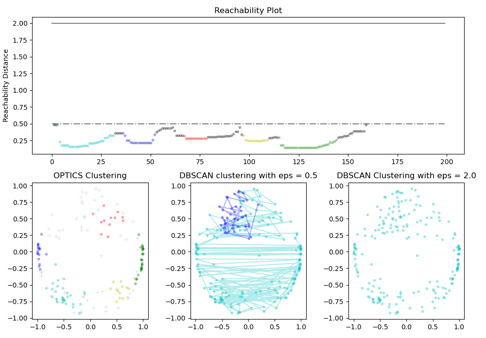
Here we are..our OPTICS model is complete…. We can print the cluster labels using optics_model.labels_
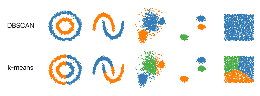
Now we will take one step further by comparing the performance of OPTICS and DBSCAN to validate DBSCAN lacks clustering in different densities
#Producing the labels according to the DBSCAN technique with eps = 0.5
labels1 = cluster_optics_dbscan(reachability = optics_model.reachability_,
core_distances = optics_model.core_distances_,ordering = optics_model.ordering_, eps = 0.5)
#Producing the labels according to the DBSCAN technique with eps = 2.0
labels2 = cluster_optics_dbscan(reachability = optics_model.reachability_,
core_distances = optics_model.core_distances_,
ordering = optics_model.ordering_, eps = 2)
#Creating a numpy array with numbers at equal spaces till
#the specified range
space = np.arange(len(X_normalized))
#Storing the reachability distance of each point
reachability = optics_model.reachability_[optics_model.ordering_]
#Visualizing the results
#Defining the framework of the visualization
plt.figure(figsize =(10, 7))
G = gridspec.GridSpec(2, 3)
ax1 = plt.subplot(G[0, :])
ax2 = plt.subplot(G[1, 0])
ax3 = plt.subplot(G[1, 1])
ax4 = plt.subplot(G[1, 2])
#Plotting the Reachability-Distance Plot
colors = ['c.', 'b.', 'r.', 'y.', 'g.']
for Class, colour in zip(range(0, 5), colors):
Xk = space[labels == Class]
Rk = reachability[labels == Class]
ax1.plot(Xk, Rk, colour, alpha = 0.3)
ax1.plot(space[labels == -1], reachability[labels == -1], 'k.', alpha = 0.3)
ax1.plot(space, np.full_like(space, 2., dtype = float), 'k-', alpha = 0.5)
ax1.plot(space, np.full_like(space, 0.5, dtype = float), 'k-.', alpha = 0.5)ax1.set_ylabel('Reachability Distance')
ax1.set_title('Reachability Plot')
#Plotting the OPTICS Clustering
colors = ['c.', 'b.', 'r.', 'y.', 'g.']
for Class, colour in zip(range(0, 5), colors):
Xk = X_normalized[optics_model.labels_ == Class]
ax2.plot(Xk.iloc[:, 0], Xk.iloc[:, 1], colour, alpha = 0.3)
ax2.plot(X_normalized.iloc[optics_model.labels_ == -1, 0],
X_normalized.iloc[optics_model.labels_ == -1, 1],'k+', alpha = 0.1)
ax2.set_title('OPTICS Clustering')
#Plotting the DBSCAN Clustering with eps = 0.5
colors = ['c', 'b', 'r', 'y', 'g', 'greenyellow']
for Class, colour in zip(range(0, 6), colors):
Xk = X_normalized[labels1 == Class]
ax3.plot(Xk.iloc[:, 0], Xk.iloc[:, 1], colour, alpha = 0.3, marker ='.')
ax3.plot(X_normalized.iloc[labels1 == -1, 0],X_normalized.iloc[labels1 == -1, 1],'k+', alpha = 0.1)
ax3.set_title('DBSCAN clustering with eps = 0.5')
#Plotting the DBSCAN Clustering with eps = 2.0
colors = ['c.', 'y.', 'm.', 'g.']
for Class, colour in zip(range(0, 4), colors):
Xk = X_normalized.iloc[labels2 == Class]
ax4.plot(Xk.iloc[:, 0], Xk.iloc[:, 1], colour, alpha = 0.3)
ax4.plot(X_normalized.iloc[labels2 == -1, 0], X_normalized.iloc[labels2 == -1, 1],'k+', alpha = 0.1)
ax4.set_title('DBSCAN Clustering with eps = 2.0')plt.tight_layout()
plt.show()
Next, we have another interesting and advanced clustering method specially used for data exploration and visualizing high-dimensional data called T-SNE

t-SNE
t-Distributed Stochastic Neighbor Embedding (t-SNE) is an unsupervised, non-linear technique primarily used for data exploration and visualizing high-dimensional data.
In other words, t-SNE is a non-linear technique for dimensionality reduction that is particularly well suited for the visualization of the high dimensional dataset. It maps the multi-dimensional data to a lower-dimensional space and attempts to find patterns in the data by identifying observed clusters based on the similarity of data points with multiple features. However, the input features are no longer identifiable and you cannot make any inference based only on the output of t-SNE. Hence it is mainly used for data exploration and visualization techniques.
Dimensionality Reduction
T-SNE vs PCA. Both use the dimensionality reduction technique. But the first thing to know is that PCA was developed in 1933 while t-SNE was developed in 2008. Second PCA is a linear dimensional reduction technique that seeks to maximize variance and preserves large pairwise distances. This can lead to poor visualization especially when dealing with non-linear manifold structures like cylindrical shape, ball, curve, etc.
t-SNE is a great tool to investigate, learn or evaluate segmentation. T-SNE gives clear separation in the data which can be used prior to using the segmentation model to select a cluster number.
However, it is not a clustering approach since it doesn’t preserve the inputs like PCA.
t-SNE has a wide range of applications in areas like climate research, computer security, bioinformatics, cancer research, fraud detection, etc. t-SNE can be used on high-dimensional data and then the output of those dimensional then become inputs to some other classification model.
Now let’s see how can we apply t-SNE
#t-SNE clustering
import swat
import pandas as pd
import numpy as np
import matplotlib.pyplot as plt
import seaborn as sns
from time import time
%matplotlib inline
#We will load a sample bioinformatics data
from bioinfokit.analys import get_data
df = get_data('digits').data
df.head()
df.shape
#run t-SNE
from sklearn.manifold import TSNE
#perplexity parameter can be changed based on the input datatset
#dataset with larger number of variables requires larger perplexity
#set this value between 5 and 50 (sklearn documentation)
#verbose=1 displays run time messages
#set n_ite sufficiently high to resolve the well stabilized cluster
#get embeddings
tsne_em = TSNE(n_components=2, perplexity=30.0, n_iter=1000, verbose=1).fit_transform(df)
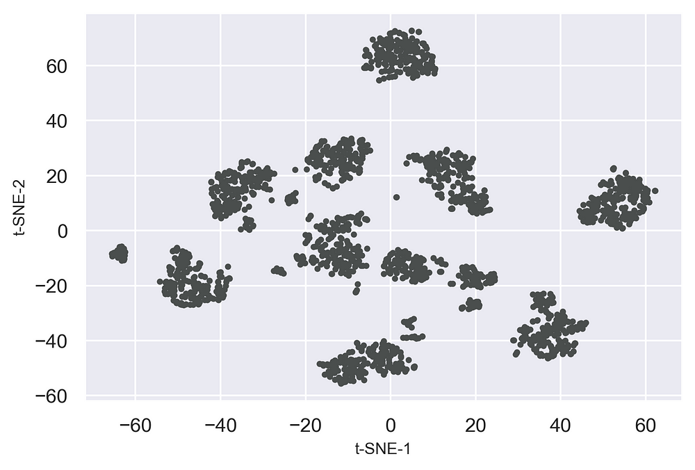
#plot t-SNE clusters
from bioinfokit.visuz import cluster
cluster.tsneplot(score=tsne_em)
Now let's add some colors
#Add Colors
#get a list of categories
color_class = df['class'].to_numpy()
cluster.tsneplot(score=tsne_em, colorlist=color_class, legendpos='upper right', legendanchor=(1.15, 1))
#Add customized colors
#get a list of categories
color_class = df['class'].to_numpy()
cluster.tsneplot(score=tsne_em, colorlist=color_class, colordot=('#713e5a', '#63a375', '#edc79b', '#d57a66', '#ca6680', '#395B50', '#92AFD7', '#b0413e', '#4381c1', '#736ced'),
    legendpos='upper right', legendanchor=(1.15, 1) )
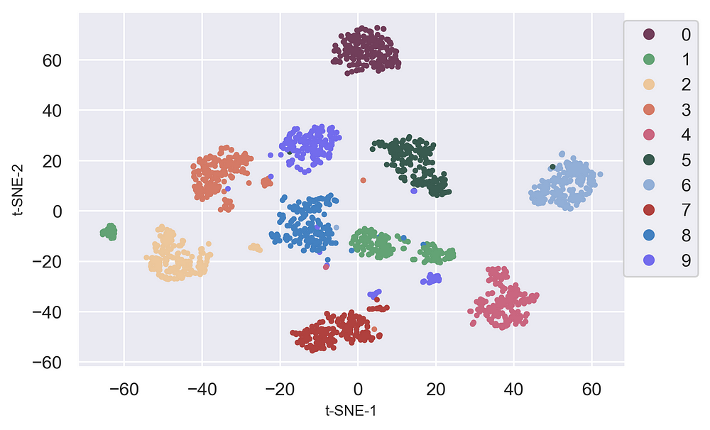
Clearly, we can see t-SNE is a great tool to investigate, learn or evaluate segmentation. T-SNE gives clear separation in the data which can be used prior to using the segmentation model to select a cluster number.
Next, we have Cure Algorithm
Cure Algorithm
Real-life implementation of the Cure Algorithm is still at an early stage due to a lack of documentation. However, I tried my best to gather as much information on the workings of the Cure Algorithm.
Cure Algorithm is a hierarchical-based clustering technique that adopts a middle ground between the centroid-based and the all-points extremes. However hierarchical clustering is clustering that stars with a single point cluster and move to merge with another cluster until the desired number of clusters are found.
· It is used for identifying the spherical and non-spherical clusters.
· It is used for discovering groups and identifying interesting distributions in the underlying data.
· Instead of using one point centroid, as in most data mining algorithms, Cure uses a set of well-defined representatives’ points, for efficiently handling the clusters and eliminating the outliers.
Differences between Cure Clustering & DBSCAN
> Cure Clustering stands for Clustering using representatives clustering.
> Noise handling is not efficient
> It is a hierarchical-based clustering technique.
> It can take care of high-dimensional datasets.
> Varying densities of the data points don’t matter in CURE clustering algorithms.
DBSCAN clustering stands for Density-Based Spatial Clustering of Applications with Noise Clustering
> It is a density-based clustering technique
> Noise handling in DBSCAN is efficient
> It doesn't work properly for the high-dimensional datasets.
> It doesn't work properly when the data pints have varying densities.
Steps of Cure Algorithm:
1.) Select target sample number ‘gfg’
2.) Choose ‘gfg’ well-scattered points in a cluster.
3.) These scattered points are shrunk towards centroid.
4.) These points are used as representatives of clusters and used in ‘Dmin’(Distance Minium) cluster merging approach. In Dmin cluster merging approach, the minimum distance from the scattered point inside the sample, when compared to other points, is considered and merged into the sample.
5.) After every such merging new sample points will be selected to present the new cluster.
6.) Cluster merging will stop until the target say ‘K’ is reached.
Next, we have another similar type of early-stage clustering method for real-life applications that is

Sub-Space Clustering.
Subspace clustering is a technique that finds clusters within different subspaces (a selection of one or more dimensions). The underlying assumption is that we can find valid clusters which are defined by only a subset of dimensions (it is not needed to have the agreement of all N features).
The resulting clusters may be overlapping both in the space of features and observations.
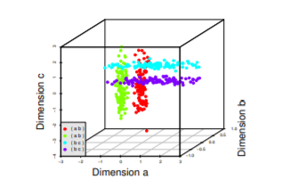
Sample dataset with four clusters, each in two dimensions with the third dimension being noise. Points from two clusters can be very close together, confusing many traditional algorithms.
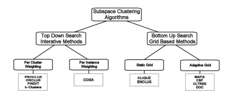
Subspace clustering can be of 2 types:
1.) Bottom-up approaches start by finding clusters in low dimensional(1D) spaces and iteratively merging them to process higher dimensional spaces (up to nth D).
2.) Top-down approaches find clusters in the full set of dimensions and evaluate the subspace of each cluster.
Subspace clustering is an unsupervised learning problem that aims at grouping data points into multiple clusters so that data points at a single cluster lie approximately on a low-dimensional linear subspace. Subspace clustering is an extension of feature selection just as with feature selection subspace clustering requires a search method and evaluation criteria but in addition subspace clustering limit the scope of evaluation criteria.
The subspace clustering algorithm localizes the search for relevant dimensions and allows them to find clusters that exist in multiple overlapping subspaces.
Subspace clustering was originally developed for computer vision problems now also been used for a movie recommendation, understanding the social network, biological dataset.
Alright, it’s been a very long chapter………….probably you might get bored in somewhere,,, sorry….I hope you have enjoyed it. I tried my best to gather and put all together from various sources in one piece so that you can get a clear picture about the possibilities with the different types of advanced clustering besides K-means and Hierarchical.

Let’s wrap up this chapter with another method that can be highly used for cluster evaluation.
Cluster Evaluation
Besides the Elbow method to find the optimal number of clusters that we already have performed in our K-means example. There is another easy way to measure and evaluate the cluster performance is by using the V-measure score function.
So to demonstrate this example we will take create 5 versions of our K-means clusters with cluster = 2,3,4,5 and 6 clusters and evaluate which one of them is performing the best.
#V-measure for evaluating Cluster performance
import pandas as pd
import matplotlib.pyplot as plt
from sklearn.cluster import KMeans
from sklearn.metrics import v_measure_score
# Loading the data
df = pd.read_csv('creditcard.csv')
# Separating the dependent and independent variables
y = df['Class']
X = df.drop('Class', axis = 1)
X.head()
# List of V-Measure Scores for different models
v_scores = []
# List of different types of covariance parameters
N_Clusters = [2, 3, 4, 5, 6]
#---------------------------------
# Building the clustering model 1
kmeans2 = KMeans(n_clusters = 2)
# Training the clustering model
kmeans2.fit(X)
# Storing the predicted Clustering labels
labels2 = kmeans2.predict(X)
# Evaluating the performance
v_scores.append(v_measure_score(y, labels2))
#-------------------------------------
# Building the clustering model 2
kmeans3 = KMeans(n_clusters = 3)
# Training the clustering model
kmeans3.fit(X)
#Storing the predicted Clustering labels
labels3 = kmeans3.predict(X)
#Evaluating the performance
v_scores.append(v_measure_score(y, labels3))
#--------------------------------------
#Building the clustering model 3
kmeans4 = KMeans(n_clusters = 4)
#Training the clustering model
kmeans4.fit(X)
#Storing the predicted Clustering labels
labels4 = kmeans4.predict(X)
#Evaluating the performance
v_scores.append(v_measure_score(y, labels4))
#--------------------------------------
#Building the clustering model 4
kmeans5 = KMeans(n_clusters = 5)
#Training the clustering model
kmeans5.fit(X)
#Storing the predicted Clustering labels
labels5 = kmeans5.predict(X)
#Evaluating the performance
v_scores.append(v_measure_score(y, labels5))
#----------------------------------------
#Building the clustering model 5
kmeans6 = KMeans(n_clusters = 6)
#Training the clustering model
kmeans6.fit(X)
#Storing the predicted Clustering labels
labels6 = kmeans6.predict(X)
#Evaluating the performance
v_scores.append(v_measure_score(y, labels6))
#-----------------------------------------------
#Step 4: Visualizing the results and comparing the performances
#Plotting a Bar Graph to compare the models
plt.bar(N_Clusters, v_scores)
plt.xlabel('Number of Clusters')
plt.ylabel('V-Measure Score')
plt.title('Comparison of different Clustering Models')
plt.show()
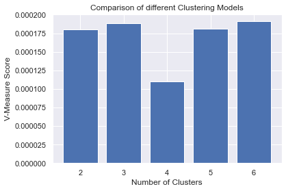
Well, you can observe what we did, we called the v_measure_score library from sklearn.metrics then we collected (append) v_measure_score from all our cluster versions and used a plot to visualize it. Thus this gives a better representation of its performance. that's it!
Well it’s a long article, i tried my best to keep it as simple as possible keeping all the important concepts intact. I hope you enjoyed and able to leverage the different types of advance clustering methods in your day to day analytical solutions.
Some of my alternative internet presences are Facebook, Instagram, Udemy, Blogger, Issuu, and more.
Also available on Quora @ https://www.quora.com/profile/Rupak-Bob-Roy
Have a good day.


Comments
Post a Comment