What is Kernel PCA? using R & Python. 4 easy lines of codes to apply the most advanced PCA for non-linearly separable data.

What is PCA first of all?
Principal Component Analysis or PCA is a statistical procedure that allows us to summarize/extract the only important data that explains the whole dataset.
Principal component analysis today is one of the most popular multivariate statistical techniques. PCA is the mother method for multivariate data analysis MVDA
It has been widely used in the areas of pattern recognition and signal processing and in statistical analysis to reduce the dimension, in simple words, to understand and extract only the important factors that explains the whole data. Thus helps in avoiding unnecessary data to be processed.
Now since we got a basic idea of what is pca.
Let’s understand what is KERNEL PCA.
Kernel PCA uses rbf radial based function to convert the non-linearly separable data to higher dimension to make it separable. So it performs better in non-linear data.
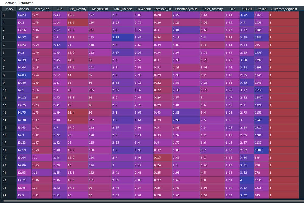
Lets load our data, define the X and Y, split the dataset into train & test and scale it to reduce the magnitude of the data points spread across. You can save this Data pre-processing template that we often need to use it before applying any model.
For this example we will use one of the famous available dataset ‘wine_quality’ were we have the key components factors of wine and its customer.
#Importing the libraries
import numpy as np
import matplotlib.pyplot as plt
import pandas as pd
#Importing the dataset
dataset = pd.read_csv('Wine.csv')
X = dataset.iloc[:, 0:13].values
y = dataset.iloc[:, 13].values
#Splitting the dataset into the Training set and Test set
from sklearn.model_selection import train_test_split
X_train, X_test, y_train, y_test = train_test_split(X, y, test_size = 0.2, random_state = 0)
#Feature Scaling
from sklearn.preprocessing import StandardScaler
sc = StandardScaler()
X_train = sc.fit_transform(X_train)
X_test = sc.transform(X_test)
Time to apply Kernel PCA
#Applying Kernel PCA
from sklearn.decomposition import KernelPCA
kpca = KernelPCA(n_components = 2, kernel = 'rbf')
X_train = kpca.fit_transform(X_train)
X_test = kpca.transform(X_test)
All we need is the n_components = 2 that is number of principal components and the kernel ‘rbf’ , rest all are same. And yes mentioned earlier ‘kpca.fit_transform‘ we don’t need to write ‘kpca.fit’ just ‘kpca.transform’ will do as python learns itself that kpca is used for transformation.
Then we will fit the 2 principal n_components in our model.
#Fitting Logistic Regression to the Training set
from sklearn.linear_model import LogisticRegression
classifier = LogisticRegression(random_state = 0)
classifier.fit(X_train, y_train)
Let’s predict our model with Test (unknown) data to get the accuracy of our model with n_components = 2
#Predicting the Test set results
y_pred = classifier.predict(X_test)
#Making the Confusion Matrix
from sklearn.metrics import confusion_matrix
cm = confusion_matrix(y_test, y_pred)
#Another evaluation Metrics
from sklearn import metrics
print('Accuracy Score:', metrics.accuracy_score(y_test, y_pred))

Nice! we have 100% accuracy of our model to our test dataset (unseen)data with perfectly separated/identified classes in confusion matrix (cm)
Let’s redo it with our simple PCA and we will compare the performance.
#Simple PCA-------------------------------------
#Splitting the dataset into the Training set and Test set
from sklearn.model_selection import train_test_split
X_train, X_test, y_train, y_test = train_test_split(X, y, test_size = 0.2, random_state = 0)
#Feature Scaling
from sklearn.preprocessing import StandardScaler
sc = StandardScaler()
X_train = sc.fit_transform(X_train)
X_test = sc.transform(X_test)
#Applying PCA
from sklearn.decomposition import PCA
pca = PCA(n_components = 2)
X_train = pca.fit_transform(X_train)
X_test = pca.transform(X_test)
#Fitting Logistic Regression to the Training set
from sklearn.linear_model import LogisticRegression
classifier = LogisticRegression(random_state = 0)
classifier.fit(X_train, y_train)
#Predicting the Test set results
y_pred = classifier.predict(X_test)
#Making the Confusion Matrix
from sklearn.metrics import confusion_matrix
cm = confusion_matrix(y_test, y_pred)
#Another evaluation Metrics
from sklearn import metrics
print('Accuracy Score:', metrics.accuracy_score(y_test, y_pred))

Oh yes! Now we have accuracy of our model 97% with 2 n_components .
So what we have learned so far? Radial based function ‘rbf’ performs better in identifying classes correctly from non-linear separable data
Rule of thumb: Use simple PCA when our data is linearly separable and used Kernel ‘rbf’ PCA when our data is complex and non-linearly separable.
Let’s put all the pieces together
#Importing the libraries
import numpy as np
import matplotlib.pyplot as plt
import pandas as pd
#Importing the dataset
dataset = pd.read_csv('Wine.csv')
X = dataset.iloc[:, 0:13].values
y = dataset.iloc[:, 13].values
#Splitting the dataset into the Training set and Test set
from sklearn.model_selection import train_test_split
X_train, X_test, y_train, y_test = train_test_split(X, y, test_size = 0.2, random_state = 0)
#Feature Scaling
from sklearn.preprocessing import StandardScaler
sc = StandardScaler()
X_train = sc.fit_transform(X_train)
X_test = sc.transform(X_test)
#Applying Kernel PCA
from sklearn.decomposition import KernelPCA
kpca = KernelPCA(n_components = 2, kernel = 'rbf')
X_train = kpca.fit_transform(X_train)
X_test = kpca.transform(X_test)
#Fitting Logistic Regression to the Training set
from sklearn.linear_model import LogisticRegression
classifier = LogisticRegression(random_state = 0)
classifier.fit(X_train, y_train)
#Predicting the Test set results
y_pred = classifier.predict(X_test)
#Making the Confusion Matrix
from sklearn.metrics import confusion_matrix
cm = confusion_matrix(y_test, y_pred)
#Another evaluation Metrics
from sklearn import metrics
print('Accuracy Score:', metrics.accuracy_score(y_test, y_pred))
#----------------------------------------
#simple PCA
#Splitting the dataset into the Training set and Test set
from sklearn.model_selection import train_test_split
X_train, X_test, y_train, y_test = train_test_split(X, y, test_size = 0.2, random_state = 0)
#Feature Scaling
from sklearn.preprocessing import StandardScaler
sc = StandardScaler()
X_train = sc.fit_transform(X_train)
X_test = sc.transform(X_test)
#Applying PCA
from sklearn.decomposition import PCA
pca = PCA(n_components = 2)
X_train = pca.fit_transform(X_train)
X_test = pca.transform(X_test)
explained_variance = pca.explained_variance_ratio_
#Fitting Logistic Regression to the Training set
from sklearn.linear_model import LogisticRegression
classifier = LogisticRegression(random_state = 0)
classifier.fit(X_train, y_train)
#Predicting the Test set results
y_pred = classifier.predict(X_test)
#Making the Confusion Matrix
from sklearn.metrics import confusion_matrix
cm = confusion_matrix(y_test, y_pred)
#Another evaluation Metrics
from sklearn import metrics
print('Accuracy Score:', metrics.accuracy_score(y_test, y_pred))
What i would suggest to use this template to apply both and see the differences if the differences are small we can use simple PCA else kernel PCA. In our case we have 0.3% difference from 1–0.97 so we can use either 3 or 2 n_components to build our model.
Now let’s perform the same Kernel PCA with R
Initially we will start with data pre-processing step, from importing the data to splitting the data into train and test set then feature scaling then we have to apply this 4 lines of code to apply kernel pca.
#Applying Kernel PCA
#install.packages('kernlab')
library(kernlab)
kpca = kpca(~., data = training_set[-14], kernel = 'rbfdot', features = 2)
training_set_pca = as.data.frame(predict(kpca, training_set))
head(training_set_pca)
training_set_pca$Customer_Segment = training_set$Customer_Segment
test_set_pca = as.data.frame(predict(kpca, test_set))
test_set_pca$Customer_Segment = test_set$Customer_Segment
first to apply kernel pca we need the package kernellab, after that Tilde ‘~’ is the separator of DV ~ IV followed by dot ‘.’ Refers to include all the columns (IVs).
Then we have to call the kernel = ‘rbfdot’ with number of principal components i.e. features = 2
Once its done we will use to predict the two most important principal components from training_set

However if you observe our newly saved results training_set_pca dosnt have the Dependent variable column so we will add it and then we will repeat the same 2 steps for test set…..done!
We have our 2 most important principal components in our train and test dataset. Now it’s time to build a model and predict its accuracy.
#Fitting our data to a svm model
library(e1071)
classifier = svm(formula = Customer_Segment ~ .,data = training_set,type = 'C-classification',kernel = 'linear')
#Predicting the Test set results
y_pred = predict(classifier, newdata = test_set[-14])
#the Confusion Matrix
cm = table(test_set[, 14], y_pred)

Nice we have perfect confusion matrix results.
Let’s put all of the R-code pieces together
#Kernel PCA
#Importing the dataset
dataset = read.csv(file.choose())
#Splitting the dataset into the Training set and Test set
#install.packages('caTools')
library(caTools)
set.seed(123)
split = sample.split(dataset$Customer_Segment, SplitRatio = 0.7)
training_set = subset(dataset, split == TRUE)
test_set = subset(dataset, split == FALSE)
nrow(training_set)/nrow(dataset)
nrow(test_set)/nrow(dataset)
#Feature Scaling [-14] refers exclude the 14th column i.e.DV
training_set[-14] = scale(training_set[-14])
test_set[-14] = scale(test_set[-14])
#Applying Kernel PCA
#install.packages('kernlab')
library(kernlab)
kpca = kpca(~., data = training_set[-14], kernel = 'rbfdot', features = 2)
training_set_pca = as.data.frame(predict(kpca, training_set))
head(training_set_pca)
training_set_pca$Customer_Segment = training_set$Customer_Segment
test_set_pca = as.data.frame(predict(kpca, test_set))
test_set_pca$Customer_Segment = test_set$Customer_Segment
#fitting data to a svm model
library(e1071)
classifier = svm(formula = Customer_Segment ~ .,
                 data = training_set,
                 type = 'C-classification',
                 kernel = 'linear')
#Predicting the Test set results
y_pred = predict(classifier, newdata = test_set[-14])
#The Confusion Matrix
cm = table(test_set[, 14], y_pred)
Now for those who wish to perform more ways of performing PCA with R programming i have a whole new course to perform various types of PCA. PCA with Big Data, PCA with Random Forest further divided into classification and regression, PCA with Generalized Boosted Models(GBM), PCA with Generalized Linear Models(GLMNET), PCA with Ensemble, PCA with fscaret and more.
Thanks for your time to read to the end. I tried my best to keep it short and simple keeping in mind to use this code in our daily life.
I hope you enjoyed it.
Feel Free to ask because “Curiosity Leads To Perfection”
My alternative internet presences, Facebook, Blogger, Linkedin, Instagram, ISSUU
Also available on Quora @ https://www.quora.com/profile/Rupak-Bob-Roy
Stay tuned for more updates.! have a good day….
~ Be Happy and Enjoy!


Comments
Post a Comment