Multi-variate LSTM Time Series Forecasting.

Hi there how’s everything going? I hope it’s good.
Well in our last article we have seen how we can apply LSTM for time series forecasting when we have a single series of sequential data. Search for these 2 articles Times Series for Regression and Univariate LSTM Time Series Forecasting from my home page. Moving ahead to our next experiment using multiple series of input to understand and forecast the next time series sequential data. We will call it Multi-variate Time Series Forecasting.
The article was originally found in ‘machine learning mastery’ by Jason. What we will try to achieve here is to simplify the complex steps with different settings and understanding to get a clear picture of the concepts to quickly solve our day-to-day time series problem.
But before that let me repeat in brief what is LSTM
Long-Strong-Term Memory (LSTM) is the next generation of Recurrent Neural Network (RNN) used in deep learning for its optimized architecture to easily capture the pattern in sequential data. The benefit of this type of network is that it can learn and remember over long sequences and does not rely on pre-specified window lagged observation as input.
In Keras, this is referred to as stateful and involves settings the “stateful” argument to “True” in the LSTM layer
What is LSTM in brief?
It is a recurrent neural network that is trained by using backpropagation through time and overcomes the vanishing gradient problem.
Now instead of having Neurons, LSTM networks have memory blocks that are connected through layers. The blocks of LSTM contain 3 non-linear gates that make it smarter than a classical neuron and a memory for sequences. The 3 types of non-linear gates include
a.) Input Gate: decides which values from the input to update the memory state.
b.) Forget Gate: handles what information to throw away from the block
c.) Output Gate: finally handles what to be in output based on input and the memory gate.
Each LSTM unit is like a mini-state machine that utilizes a ”memory” cell that may maintain its state value over a longer time, where the gates of the units have weights that are learned during the training procedure.
There are tons of articles available on the internet about the workings of LSTM even the math behind LSTM. So here I will concentrate more on the quicker practical implementation of LSTM for our day-to-day problems.
Let’s get started.
First is the data pre-processing step where we have to give structure the data into supervised learning that is X and Y format.
In simple words, it identifies the strength and values of the relationship (positive/negative impact and the values derived is called quantification of impact) between one dependent variable(Y) and a series of other independent variables X
For this example, we have retail sales time series data recorded over a period of time.
Now as u know supervised learning requires X & Y independent and dependent variables for the algorithm to learn /train, so we will first convert our data into such a format
Assume we have sales data. What we will do is we will first take the sales data(t) in our first column then the second column will have the next month's (t+1)sales data that we will use to predict. Remember X & Y independent and dependent variable format where we use Y to predict the data.
Now we will replicate the same if we have more columns.
Let’s take an example of weather conditions data set where we will have attributes/ columns/ like pollution, dew, temp, wind speed, snow, rain. Now we will use the Multivariate LSTM time series forecasting technique to predict the pollution for the next hours based on pollution, dew, temp, wind speed, snow, rain conditions.
We will use series to supervised function to frame our dataset/variables of the dataset into t+1 and t format
#transform series to supervised learning
def series_to_supervised(data, n_in=1, n_out=1, dropnan=True):
n_vars = 1 if type(data) is list else data.shape[1]
df = DataFrame(data)
cols, names = list(), list()
#input sequence (t-n, ... t-1)
for i in range(n_in, 0, -1):
cols.append(df.shift(i))
names += [('var%d(t-%d)' % (j+1, i)) for j in range(n_vars)]
#forecast sequence (t, t+1, ... t+n)
for i in range(0, n_out):
cols.append(df.shift(-i))
if i == 0:
names += [('var%d(t)' % (j+1)) for j in range(n_vars)]
else:
names += [('var%d(t+%d)' % (j+1, i)) for j in range(n_vars)]
#put it all together
agg = concat(cols, axis=1)
agg.columns = names
#drop rows with NaN values
if dropnan:
agg.dropna(inplace=True)
return agg
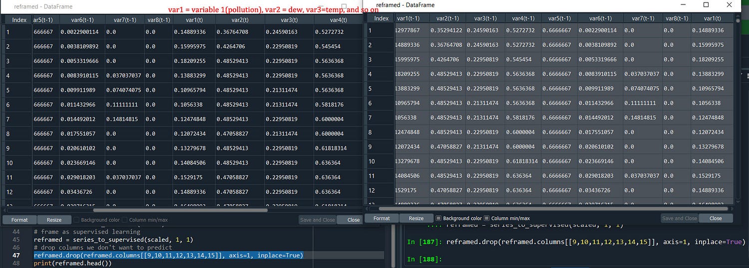
Here is it after converting where we have all the variables in var(t-1) and var (t) is the same meaning as (t) (t+1) where we are using 1 step back to format it into X and Y variable.

And yes since we will predict the pollution we will drop all other (t) columns, the values that we see are normalized scaled values. Few more things that we can experiment with transform our dataset to stationary values by differencing
Our dataset is not stationary. This means that there is a structure in the data that is dependent on time. We can see there is an increasing trend in the data. Stationary data is easier to model and will very likely result in more skillful forecasts. The trend can be removed from observations, then use for forecasts later we can scale it to the original value for prediction.
We can easily remove a trend by differencing the data with diff() function from pandas that are the observations from the previous time step (t-1) is subtracted from the current observation(t). This will give us a series of difference
Now it’s time to define the model…
#define the network
model = Sequential()
model.add(LSTM(15, input_shape=(train_X.shape[1], train_X.shape[2])))
model.add(Dense(1))
model.compile(loss='mae', optimizer='adam',metrics=["accuracy"])
#fit network
trained = model.fit(train_X, train_y, epochs=30, batch_size=28, validation_data=(test_X, test_y), verbose=1, shuffle=False)
We will use Sequential API to define the network. Then the shape of the input data must be specified in the LSTM layer using the “batch_input_shape” argument and 15 is the number of neurons also called memory units or blocks.
Then we have 1 neuron/block that is our output layer Dense(1). In the compiling network, we must specify a loss function and optimization algorithm to calculate the loss and weight. Verbose refers to the display of progress while training the model.
By default, the samples within an epoch are shuffled prior to being exposed to the network, we will disable the shuffling of samples by settings “shuffle” to “False”
We can also try a different numbers of iterations/epochs to train our model, however unnecessarily increasing the epoch value will not necessarily improve the result.
Batch size is the number of values that we can use at a time to train. Different batch size settings also result in different results.
Let’s wrap up all of these and execute.
from math import sqrt
from numpy import concatenate
from matplotlib import pyplot
from pandas import read_csv
from pandas import DataFrame
from pandas import concat
from sklearn.preprocessing import MinMaxScaler
from sklearn.preprocessing import LabelEncoder
from sklearn.metrics import mean_squared_error
from keras.models import Sequential
from keras.layers import Dense
from keras.layers import LSTM

# convert series to supervised learning
def series_to_supervised(data, n_in=1, n_out=1, dropnan=True):
 n_vars = 1 if type(data) is list else data.shape[1]
 df = DataFrame(data)
 cols, names = list(), list()
 # input sequence (t-n, ... t-1)
 for i in range(n_in, 0, -1):
  cols.append(df.shift(i))
  names += [('var%d(t-%d)' % (j+1, i)) for j in range(n_vars)]
 # forecast sequence (t, t+1, ... t+n)
 for i in range(0, n_out):
  cols.append(df.shift(-i))
  if i == 0:
   names += [('var%d(t)' % (j+1)) for j in range(n_vars)]
  else:
   names += [('var%d(t+%d)' % (j+1, i)) for j in range(n_vars)]
 # put it all together
 agg = concat(cols, axis=1)
 agg.columns = names
 # drop rows with NaN values
 if dropnan:
  agg.dropna(inplace=True)
 return agg

# load dataset
dataset = read_csv('pollution.csv', header=0, index_col=0)
values = dataset.values
#Encode Character Values
encoder = LabelEncoder()
values[:,4] = encoder.fit_transform(values[:,4])
# ensure all data is float
values = values.astype('float32')
# normalize features
scaler = MinMaxScaler(feature_range=(0, 1)) #(dew and temp column is in negative)
scaled = scaler.fit_transform(values)
# frame as supervised learning
reframed = series_to_supervised(scaled, 1, 1)
# drop columns we don't want to predict
reframed.drop(reframed.columns[[9,10,11,12,13,14,15]], axis=1, inplace=True)
print(reframed.head())
# split into input and outputs
X = values[:, :8]
y = values[:, :-8]
# Splitting the dataset into the Training set and Test set
from sklearn.model_selection import train_test_split
train_X, test_X,train_y, test_y = train_test_split(X, y, test_size = 0.2, random_state = 0)
# reshape input to be 3D [samples, timesteps, features] 8features i.e. 8 columns
train_X = train_X.reshape((train_X.shape[0], 1, train_X.shape[1]))
test_X = test_X.reshape((test_X.shape[0], 1, test_X.shape[1]))
print(train_X.shape, train_y.shape, test_X.shape, test_y.shape)

#define the network
model = Sequential()
model.add(LSTM(15, input_shape=(train_X.shape[1], train_X.shape[2])))
model.add(Dense(1))
model.compile(loss='mae', optimizer='adam',metrics=["accuracy"])
# fit network
trained = model.fit(train_X, train_y, epochs=30, batch_size=28, validation_data=(test_X, test_y), verbose=1, shuffle=False)
# plot history
pyplot.plot(trained.history['loss'], label='train')
pyplot.plot(trained.history['val_loss'], label='test')
pyplot.legend()
pyplot.show()

# make a prediction
yhat = model.predict(test_X)
test_X = test_X.reshape((test_X.shape[0], test_X.shape[2]))
# invert scaling for forecast
inv_yhat = concatenate((yhat, test_X[:, 1:]), axis=1)
inv_yhat = scaler.inverse_transform(inv_yhat)
inv_yhat = inv_yhat[:,0]
# invert scaling for actual
test_y = test_y.reshape((len(test_y), 1))
inv_y = concatenate((test_y, test_X[:, 1:]), axis=1)
inv_y = scaler.inverse_transform(inv_y)
inv_y = inv_y[:,0]
# calculate RMSE
rmse = sqrt(mean_squared_error(inv_y, inv_yhat))
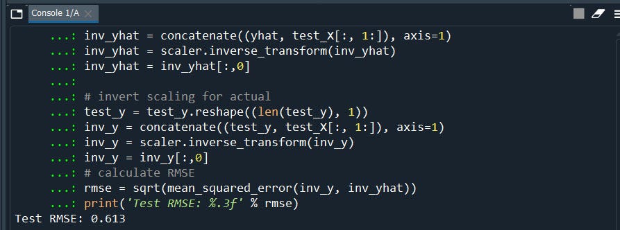
print('Test RMSE: %.3f' % rmse)


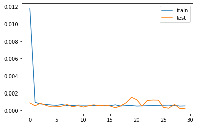
Well, we have RMSE 0.61 that good the lower the value the better our model is. Our trained model is fitting well in our test data set. Model is overfitted when val_loss(test) is more than train loss(train)
Note: loss is the error evaluated during training a model, val_loss is the error during validation.
I hope I’m to able re-frame the Multi-variate LSTM concepts. Feel Free to discuss any new concepts or innovative ways to use LSTMs for our day-to-day solutions.
Next, I’m going to write deeper about Multivariate Multi-Step LSTM Time Series Forecasting and replicate the same example above to validate its better performance on Time Series Data. Stay Tune!
I hope you enjoyed it.
Some of my alternative internet presences are Facebook, Instagram, Udemy, Blogger, Issuu, and more.
Also available on Quora @ https://www.quora.com/profile/Rupak-Bob-Roy
Have a good day.

Comments
Post a Comment