Multi-Step LSTM Time Series Forecasting ~Apply Advanced Deep Learning Multi-Step Time Series Forecasting with the help of this template.

Hi there, how are you doing, I hope it’s great!
In my last article, we used Multi-variate LSTM that is multiple inputs for LSTM to forecast Time Series data.
This time we will use take one step further with step-wise forecasting. For this example, we will forecast 3 months.
The article was originally found in ‘machine learning mastery’ by Jason. What we will try to achieve here is to simplify the complex steps with different settings and understanding to get a clear picture of the concepts to quickly solve our day-to-day time series problem.
But before that let me repeat in brief what is LSTM
Long-Strong-Term Memory (LSTM) is the next generation of Recurrent Neural Network (RNN) used in deep learning for its optimized architecture to easily capture the pattern in sequential data. The benefit of this type of network is that it can learn and remember over long sequences and does not rely on pre-specified window lagged observation as input.
In Keras, this is referred to as stateful and involves settings the “stateful” argument to “True” in the LSTM layer
What is LSTM in brief?
It is a recurrent neural network that is trained by using backpropagation through time and overcomes the vanishing gradient problem.
Now instead of having Neurons, LSTM networks have memory blocks that are connected through layers. The blocks of LSTM contain 3 non-linear gates that make it smarter than a classical neuron and a memory for sequences. The 3 types of non-linear gates include
a.) Input Gate: decides which values from the input to update the memory state.
b.) Forget Gate: handles what information to throw away from the block
c.) Output Gate: finally handles what to be in output based on input and the memory gate.
Each LSTM unit is like a mini-state machine that utilizes a ”memory” cell that may maintain its state value over a longer time, where the gates of the units have weights that are learned during the training procedure.
There are tons of articles available on the internet about the workings of LSTM even the math behind LSTM. So here I will concentrate more on the quicker practical implementation of LSTM for our day-to-day problems.
Let’s get started.
First is the data pre-processing step where we have to give structure the data into supervised learning that is X and Y format.
In simple words, it identifies the strength and values of the relationship (positive/negative impact and the values derived is called quantification of impact) between one dependent variable(Y) and a series of other independent variables X
For this example, we have retail sales time series data recorded over a period of time.
Now as u know supervised learning requires X & Y independent and dependent variables for the algorithm to learn /train, so we will first convert our data into such a format
Assume we have sales data. What we will do is we will first take the sales data(t) in our first column then the second column will have the next month's (t+1)sales data that we will use to predict. Remember X & Y independent and dependent variable format where we use Y to predict the data.
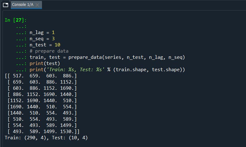
Now we will replicate the same if we have more columns. And since we are predicting for the next 3 months we will take t, t+1,t+2
Let me show you the dataset how it will be.

Now since we have our data ready to train our model using lstm we will straight away move on to the full code to make it quick and easier to understand its components.
from pandas import DataFrame
from pandas import Series
from pandas import concat
from pandas import read_csv
from sklearn.metrics import mean_squared_error
from sklearn.preprocessing import MinMaxScaler
from keras.models import Sequential
from keras.layers import Dense
from keras.layers import LSTM
from math import sqrt
from matplotlib import pyplot
from numpy import array
#a.) convert time series into supervised learning problem
def series_to_supervised(data, n_in=1, n_out=1, dropnan=True):
 n_vars = 1 if type(data) is list else data.shape[1]
 df = DataFrame(data)
 cols, names = list(), list()
 # input sequence (t-n, ... t-1)
 for i in range(n_in, 0, -1):
  cols.append(df.shift(i))
  names += [('var%d(t-%d)' % (j+1, i)) for j in range(n_vars)]
 # forecast sequence (t, t+1, ... t+n)
 for i in range(0, n_out):
  cols.append(df.shift(-i))
  if i == 0:
   names += [('var%d(t)' % (j+1)) for j in range(n_vars)]
  else:
   names += [('var%d(t+%d)' % (j+1, i)) for j in range(n_vars)]
 # put it all together
 agg = concat(cols, axis=1)
 agg.columns = names
 # drop rows with NaN values
 if dropnan:
  agg.dropna(inplace=True)
 return agg

#b.) create a differenced series
def difference(dataset, interval=1):
 diff = list()
 for i in range(interval, len(dataset)):
  value = dataset[i] - dataset[i - interval]
  diff.append(value)
 return Series(diff)

#c.) transform series into train and test sets for supervised learning
def prepare_data(series, n_test, n_lag, n_seq):
 # extract raw values
 raw_values = series.values
 # transform data to be stationary
 diff_series = difference(raw_values, 1)
 diff_values = diff_series.values
 diff_values = diff_values.reshape(len(diff_values), 1)
 # rescale values to -1, 1
 scaler = MinMaxScaler(feature_range=(-1, 1))
 scaled_values = scaler.fit_transform(diff_values)
 scaled_values = scaled_values.reshape(len(scaled_values), 1)
 # transform into supervised learning problem X, y
 supervised = series_to_supervised(scaled_values, n_lag, n_seq)
 supervised_values = supervised.values
 # split into train and test sets
 train, test = supervised_values[0:-n_test], supervised_values[-n_test:]
 return scaler, train, test

#d.) Define the LSTM network
def fit_lstm(train, n_lag, n_seq, n_batch, nb_epoch, n_neurons):
 # reshape training into [samples, timesteps, features]
 X, y = train[:, 0:n_lag], train[:, n_lag:]
 X = X.reshape(X.shape[0], 1, X.shape[1])
 # design network
 model = Sequential()
 model.add(LSTM(n_neurons, batch_input_shape=(n_batch, X.shape[1], X.shape[2]), stateful=True))
 model.add(Dense(y.shape[1]))
 model.compile(loss='mean_squared_error', optimizer='adam',metric=["accuracy"])
 # fit network
 for i in range(nb_epoch):
  model.fit(X, y, epochs=1, batch_size=n_batch, verbose=1, shuffle=False)
  model.reset_states()
 return model

#e.) forecast with an LSTM,
def forecast_lstm(model, X, n_batch):
 # reshape input pattern to [samples, timesteps, features]
 X = X.reshape(1, 1, len(X))
 # make forecast
 forecast = model.predict(X, batch_size=n_batch)
 # convert to array
 return [x for x in forecast[0, :]]

#f.)  evaluate the persistence model
def make_forecasts(model, n_batch, train, test, n_lag, n_seq):
 forecasts = list()
 for i in range(len(test)):
  X, y = test[i, 0:n_lag], test[i, n_lag:]
  # make forecast
  forecast = forecast_lstm(model, X, n_batch)
  # store the forecast
  forecasts.append(forecast)
 return forecasts

#g.) invert differenced forecast
def inverse_difference(last_ob, forecast):
 # invert first forecast
 inverted = list()
 inverted.append(forecast[0] + last_ob)
 # propagate difference forecast using inverted first value
 for i in range(1, len(forecast)):
  inverted.append(forecast[i] + inverted[i-1])
 return inverted

#h.) inverse data transform on forecasts
def inverse_transform(series, forecasts, scaler, n_test):
 inverted = list()
 for i in range(len(forecasts)):
  # create array from forecast
  forecast = array(forecasts[i])
  forecast = forecast.reshape(1, len(forecast))
  # invert scaling
  inv_scale = scaler.inverse_transform(forecast)
  inv_scale = inv_scale[0, :]
  # invert differencing
  index = len(series) - n_test + i - 1
  last_ob = series.values[index]
  inv_diff = inverse_difference(last_ob, inv_scale)
  # store
  inverted.append(inv_diff)
 return inverted

#i.) evaluate the model with RMSE
def evaluate_forecasts(test, forecasts, n_lag, n_seq):
 for i in range(n_seq):
  actual = [row[i] for row in test]
  predicted = [forecast[i] for forecast in forecasts]
  rmse = sqrt(mean_squared_error(actual, predicted))
  print('t+%d RMSE: %f' % ((i+1), rmse))

#j.) plot the forecasts
def plot_forecasts(series, forecasts, n_test):
 # plot the entire dataset in blue
 pyplot.plot(series.values)
 # plot the forecasts in red
 for i in range(len(forecasts)):
  off_s = len(series) - n_test + i - 1
  off_e = off_s + len(forecasts[i]) + 1
  xaxis = [x for x in range(off_s, off_e)]
  yaxis = [series.values[off_s]] + forecasts[i]
  pyplot.plot(xaxis, yaxis, color='red')
 # show the plot
 pyplot.show()
# load the dataset
series = read_csv('sales_year.csv', usecols=[1], engine='python')
# configure
n_lag = 1
n_seq = 3
n_test = 10
n_epochs = 1500
n_batch = 1
n_neurons = 50
#prepare data
scaler, train, test = prepare_data(series, n_test, n_lag, n_seq)
#fit model
model = fit_lstm(train, n_lag, n_seq, n_batch, n_epochs, n_neurons)
#forecasts
forecasts = make_forecasts(model, n_batch, train, test, n_lag, n_seq)
#inverse transform forecasts and test
forecasts = inverse_transform(series, forecasts, scaler, n_test+2)
actual = [row[n_lag:] for row in test]
actual = inverse_transform(series, actual, scaler, n_test+2)
#evaluate forecasts
evaluate_forecasts(actual, forecasts, n_lag, n_seq)
#plot forecasts
plot_forecasts(series, forecasts, n_test+2)
First, we will call all the important libraries than
a) we will define functions to convert times series into supervised learning problems.
b) The next step is to convert the time series data to Stationary. And our ‘sales_year.csv’ data is not stationary.
This means that there is a structure in the data that is dependent on time. We can see there is an increasing trend in the data
Stationary data is easier to model and will very likely result in more skillful forecasts. The trend can be removed from observations, then use for forecasts later we can scale it to the original value for prediction.
We can easily remove a trend by differencing the data with diff() function from pandas that are the observations from the previous time step (t-1) is subtracted from the current observation(t). This will give us a series of differences.
c.) Now it's time to normalize/scale the data.
LSTMs are a bit sensitive to the widespread scale of data. Even in all deep learning methods scaling the data range of -1 to 1 before fitting it to our algorithm is good practice that helps the algorithm to work faster and effectively. And yes scaling the data will not lose its original meaning from the data. We also call this a Normalization using the MinMaxScaler pre-processing class function. Even the default activation function for LSTMS is the hyperbolic tangent (tanh) which outputs values between -1 and 1 which is the preferred range for the time series data.
Then we will split the data into train and test.
d.) It's time to deploy LSTM.
By default, an LSTM layer in Keras maintains a state between data within one batch. A batch of data is a fixed-sized number of rows from the training dataset that defines how many patterns to process before updating the weights of the network. By default State in the LSTM layer between batches is cleared. Therefore we must make the LSTM stateful. This gives us fine-grained control over when the state of the LSTM layer is cleared
LSTM network expects the input data(X) to be [samples, time steps, features] format.
batch_input_shape=(n_batch, X.shape[1], X.shape[2])
The batch size of 1 must be used since we require prediction to be made at each time step of the test dataset.
And the number of neurons also called memory units or blocks. Then we have 1 output layer Dense(1). In the compiling network, we must specify a loss function and optimization algorithm to calculate the loss and weight. This is just our regular LSTM stuffs that we have learned from our previous chapter.
Now e.) and f.) are the functions to predict the next 3-time sequence then g.) and h.) is to inverse the forecast value to our original data set value. Remember we have scaled value with MinMaxScaler and then differenced series to remove the trend ‘Stationary’
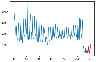
Finally i.) we will calculate the Root Mean Square Error RMSE to understand the accuracy level and at the same time j.) we will plot our 3-month forecast
Running the code will give you the plot and the RMSE score.
Output:
t+1 RMSE: 194.077577
t+2 RMSE: 293.865938
t+3 RMSE: 334.348398
We can notice that RMSE does not become progressively worse with each forecast. This is because that t+2 is easier to forecast than t+1

We can notice that RMSE does not become progressively worse with each forecast. This is because that t+2 is easier to forecast than t+1
The plot also depicts the model needs improvement over the LSTM network.
I hope I’m able to simplify the concept. There’s plenty of room for improvement let me know if you are able to improve the model.
Some of my alternative internet presences are Facebook, Instagram, Udemy, Blogger, Issuu, and more.
Also available on Quora @ https://www.quora.com/profile/Rupak-Bob-Roy
Have a good day!

Comments
Post a Comment