Grid Search For ML & Deep Learning Model
Full guide to grid search on finding the best hyperparameters for our regular ml models to deep learning models

Hi how are you doing, I hope its great.
Today we will look into ways to find the best parameters for our Machine Learning models as well as for our Deep Learning models. Finding the best parameters by manual tuning is tedious process and time consuming as it contains so many parameters to be test over and over again. Well it’s a time consuming and not productive. So to overcome this issue we will look into a method ‘GRID SEARCH’ to automate the task of finding the best model parameters for us.
We will divide this into 2 section: a) Grid Search for finding the best hyper-parameters for our machine learning model b.) Grid Search for Deep Learning models.
Let’s start with a) Grid Search for machine learning models
For this example we will use data that can be used for credit scoring. In this dataset we have details like income, age, loan, and defaulter in 1-yes or 0-no. Let’s first make our simple machine learning model predict whether we should approve for credit or not.
#Importing the libraries
import numpy as np
import matplotlib.pyplot as plt
import pandas as pd
#Importing the dataset
dataset = pd.read_csv('credit_data.csv', sep=",")
#drop the missing values
dataset = dataset.dropna()
X = dataset.iloc[:,1:4].values
y = dataset.iloc[:, 4].values
First, we load the data and define the X-dependent variables( 0 -3rd column) and y-independent variables (defaulter 4th column)
#----------------------------------------------------------
#Splitting the dataset into the Training set and Test set
from sklearn.model_selection import train_test_split
X_train, X_test, y_train, y_test = train_test_split(X, y, test_size = 0.25, random_state = 0)
from sklearn.preprocessing import StandardScaler
sc = StandardScaler()
X_train = sc.fit_transform(X_train)
X_test = sc.transform(X_test)
#Fitting SVM to the Training set
from sklearn.svm import SVC
svm_model = SVC(kernel = 'linear', random_state = 0)
svm_model.fit(X_train, y_train)
#Predicting the Test set results
y_pred = svm_model.predict(X_test)
#We can also compare the actual versus predicted
df = pd.DataFrame({'Actual': y_test.flatten(), 'Predicted': y_pred.flatten()})
df
#Making the Confusion Matrix
from sklearn.metrics import confusion_matrix
cm = confusion_matrix(y_test, y_pred)
#evaluation Metrics
from sklearn import metrics
print('Accuracy Score:', metrics.accuracy_score(y_test, y_pred))
print('Balanced Accuracy Score:', metrics.balanced_accuracy_score(y_test, y_pred))
print('Average Precision:',metrics.average_precision_score(y_test, y_pred))
Then we will split the data into train and test, scale our data before we fit our model. For this example, we will use Support Vector Machine (SVM) which is one of the powerful classifiers with default parameters.
With evaluation Metrics of the model we get
Accuracy Score: 0.948
Balanced Accuracy Score: 0.8707788671023965
Average Precision: 0.6733662239089184
It’s time to use the Grid Search to automate the search of best parameters of our svm_model.
#Applying k-Fold Cross Validation
from sklearn.model_selection import cross_val_score
accuracies = cross_val_score(estimator = svm_model, X = X_train, y = y_train, cv = 10)
accuracies.mean()
accuracies.std()
#Applying Grid Search to find the best model and the best parameters
from sklearn.model_selection import GridSearchCV
parameters = [{'C': [1, 10, 100, 1000], 'kernel': ['linear']},{'C': [1, 10, 100, 1000], 'kernel': ['rbf'], 'gamma': [0.1, 0.2, 0.3, 0.4, 0.5, 0.6, 0.7, 0.8, 0.9]}]grid_search = GridSearchCV(estimator = svm_model,param_grid = parameters,scoring = 'accuracy',cv = 10)
grid_search = grid_search.fit(X_train, y_train)
best_accuracy = grid_search.best_score_
best_parameters = grid_search.best_params_
Well what we got here is pretty much creating a list of parameters and feeding it into GridSearch with cross validation cv= 10 and we have
best_parameters
Out[165]: {'C': 1000, 'gamma': 0.9, 'kernel': 'rbf'}
best_accuracy
Out[166]: 0.9953243847874722
Alright! Let’s see if these Hyper-parameters can improve the accuracy of our model.
#Fitting SVM to the Training set
from sklearn.svm import SVC
svm_model = SVC(kernel = 'rbf', C = 1000, gamma = 0.9, random_state = 0)
svm_model.fit(X_train, y_train)
#Predicting the Test set results
y_pred = svm_model.predict(X_test)
#We can also compare the actual versus predicted
df = pd.DataFrame({'Actual': y_test.flatten(), 'Predicted': y_pred.flatten()})
df
#Making the Confusion Matrix
from sklearn.metrics import confusion_matrix
cm = confusion_matrix(y_test, y_pred)
#evaluation Metrics
from sklearn import metrics
print('Accuracy Score:', metrics.accuracy_score(y_test, y_pred))
print('Balanced Accuracy Score:', metrics.balanced_accuracy_score(y_test, y_pred))
print('Average Precision:',metrics.average_precision_score(y_test, y_pred))
Accuracy Score: 0.994
Balanced Accuracy Score: 0.9903322440087146
Average Precision: 0.9587348678601876
Nice! It did improve from 0.94 to 0.99. You can use these codes as a template with a few modifications like the list of parameters for different types of classifiers and to know the parameters you can simply select the classifier name ‘svm’ + press ‘ctrl’ + ‘i’
Let’s me put all of the pieces together.
#Importing the libraries
import numpy as np
import matplotlib.pyplot as plt
import pandas as pd
#Importing the dataset
dataset = pd.read_csv('credit_data.csv', sep=",")
#drop the missing values
dataset = dataset.dropna()
X = dataset.iloc[:,1:4].values
y = dataset.iloc[:, 4].values
#---------------------------------------------------------
#Splitting the dataset into the Training set and Test set
from sklearn.model_selection import train_test_split
X_train, X_test, y_train, y_test = train_test_split(X, y, test_size = 0.25, random_state = 0)
from sklearn.preprocessing import StandardScaler
sc = StandardScaler()
X_train = sc.fit_transform(X_train)
X_test = sc.transform(X_test)
#Fitting SVM to the Training set
from sklearn.svm import SVC
svm_model = SVC(kernel = 'linear', random_state = 0)
svm_model.fit(X_train, y_train)
#Predicting the Test set results
y_pred = svm_model.predict(X_test)
#We can also compare the actual versus predicted
df = pd.DataFrame({'Actual': y_test.flatten(), 'Predicted': y_pred.flatten()})
df
#Making the Confusion Matrix
from sklearn.metrics import confusion_matrix
cm = confusion_matrix(y_test, y_pred)
#evaluation Metrics
from sklearn import metrics
print('Accuracy Score:', metrics.accuracy_score(y_test, y_pred))
print('Balanced Accuracy Score:', metrics.balanced_accuracy_score(y_test, y_pred))
print('Average Precision:',metrics.average_precision_score(y_test, y_pred))
#########################################################
#Applying k-Fold Cross Validation
from sklearn.model_selection import cross_val_score
accuracies = cross_val_score(estimator = svm_model, X = X_train, y = y_train, cv = 10)
accuracies.mean()
accuracies.std()
#Applying Grid Search to find the best model and the best parameters
from sklearn.model_selection import GridSearchCV
parameters = [{'C': [1, 10, 100, 1000], 'kernel': ['linear']},
              {'C': [1, 10, 100, 1000], 'kernel': ['rbf'], 'gamma': [0.1, 0.2, 0.3, 0.4, 0.5, 0.6, 0.7, 0.8, 0.9]}]
grid_search = GridSearchCV(estimator = svm_model,
                           param_grid = parameters,
                           scoring = 'accuracy',
                           cv = 10)
grid_search = grid_search.fit(X_train, y_train)
best_accuracy = grid_search.best_score_
best_parameters = grid_search.best_params_
###########################################################
#Lets retry our model with the new paramters
#Fitting SVM to the Training set
from sklearn.svm import SVC
svm_model = SVC(kernel = 'rbf', C = 1000, gamma = 0.9, random_state = 0)
svm_model.fit(X_train, y_train)
#Predicting the Test set results
y_pred = svm_model.predict(X_test)
#We can also compare the actual versus predicted
df = pd.DataFrame({'Actual': y_test.flatten(), 'Predicted': y_pred.flatten()})
df
#Making the Confusion Matrix
from sklearn.metrics import confusion_matrix
cm = confusion_matrix(y_test, y_pred)
#evaluation Metrics
from sklearn import metrics
print('Accuracy Score:', metrics.accuracy_score(y_test, y_pred))
print('Balanced Accuracy Score:', metrics.balanced_accuracy_score(y_test, y_pred))
print('Average Precision:',metrics.average_precision_score(y_test, y_pred))
I hope you liked this tutorial. Next, we will see how to use Grid Search for Deep Learning Methods.

Grid Search for Deep Learning
First we will create a simple Neural Network with default parameters and later we will improve over time using Grid Search
For this example, we will use a Churn modeling dataset with details having gender, credits core, age, tenure, location, etc. A common churn modeling data set that we already have come across.
#Importing the libraries
import numpy as np
import matplotlib.pyplot as plt
import pandas as pd
#Importing the dataset
dataset = pd.read_csv('Churn_Modelling.csv')
X = dataset.iloc[:, 3:13].values
y = dataset.iloc[:, 13].values
#Encoding categorical data
from sklearn.preprocessing import LabelEncoder, OneHotEncoder
from sklearn.compose import ColumnTransformer
#country column
ct = ColumnTransformer([("Country", OneHotEncoder(), [1])], remainder = 'passthrough')
X = ct.fit_transform(X)
#to avoid dummy variable trap
X = X[:, 1:]
#Male/Female
labelencoder_X = LabelEncoder()
X[:, 3] = labelencoder_X.fit_transform(X[:, 3])
#Splitting the dataset into the Training set and Test set
from sklearn.model_selection import train_test_split
X_train, X_test, y_train, y_test = train_test_split(X, y, test_size = 0.2, random_state = 0)
#Feature Scaling
from sklearn.preprocessing import StandardScaler
sc = StandardScaler()
X_train = sc.fit_transform(X_train)
X_test = sc.transform(X_test)
#Creating the Ann model
#Importing the Keras libraries and packages
import keras
from keras.models import Sequential
from keras.layers import Dense
#Initialising the ANN
classifier = Sequential()
#Adding the input layer and the first hidden layer
classifier.add(Dense(units = 6, kernel_initializer = 'uniform', activation = 'relu', input_dim = 11))
#Adding the second hidden layer
classifier.add(Dense(units = 6, kernel_initializer = 'uniform', activation = 'relu'))
#Adding the output layer
classifier.add(Dense(units = 1, kernel_initializer = 'uniform', activation = 'sigmoid'))
#Compiling the ANN
classifier.compile(optimizer = 'adam', loss = 'binary_crossentropy', metrics = ['accuracy'])
#Fitting the ANN to the Training set
classifier.fit(X_train, y_train, batch_size = 10, epochs = 100)
#Part 3 - Making the predictions and evaluating the model
#Predicting the Test set results
y_pred = classifier.predict(X_test)
y_pred = (y_pred > 0.5)
#Making the Confusion Matrix
from sklearn.metrics import confusion_matrix
cm = confusion_matrix(y_test, y_pred)
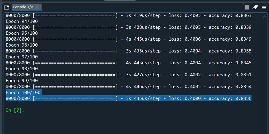
We have an Accuracy Score of 83.5% remember that. Now let’s
- Grid Search the batch_size and epochs then followed by
- Grid Search Optimizer
- Grid Search Learning Rate and Momentum
- Network Weight Initialization
- Neuron Activation
- Tune Dropout Regularization
- Tune Drop out Regularization
- Tune Number of Neurons
#scikit-learn to grid search the batch size and epochs
import numpy
from sklearn.model_selection import GridSearchCV
from keras.models import Sequential
from keras.layers import Dense
from keras.wrappers.scikit_learn import KerasClassifier
#Function to create model, required for KerasClassifier
def create_model():
model=Sequential()
model.add(Dense(units = 6, kernel_initializer='uniform',activation = 'relu',input_dim = 11))
model.add(Dense(units = 6, kernel_initializer='uniform',activation = 'relu'))
model.add(Dense(units = 1, kernel_initializer = 'uniform', activation = 'sigmoid'))
#compile model
model.compile(optimizer = 'adam',loss = 'binary_crossentropy', metrics = ['accuracy'])
return model
#Importing the libraries
import numpy as np
import pandas as pd
#Importing the dataset
dataset = pd.read_csv('Churn_Modelling.csv')
X = dataset.iloc[:, 3:13].values
y = dataset.iloc[:, 13].values
#Encoding categorical data
from sklearn.preprocessing import LabelEncoder, OneHotEncoder
from sklearn.compose import ColumnTransformer
#country column
ct = ColumnTransformer([("Country", OneHotEncoder(), [1])], remainder = 'passthrough')
X = ct.fit_transform(X)
#to avoid dummy variable trap
X = X[:, 1:]
#Male/Female
labelencoder_X = LabelEncoder()
X[:, 3] = labelencoder_X.fit_transform(X[:, 3])
#Splitting the dataset into the Training set and Test set
from sklearn.model_selection import train_test_split
X_train, X_test, y_train, y_test = train_test_split(X, y, test_size = 0.2, random_state = 0)
#Feature Scaling
from sklearn.preprocessing import StandardScaler
sc = StandardScaler()
X_train = sc.fit_transform(X_train)
X_test = sc.transform(X_test)
Till here it’s the our regular data pre-processing step, now let’s define a parameter list for batch size and epochs
model = KerasClassifier(build_fn=create_model, verbose=1)
#define the grid search parameters
batch_size = [10, 20, 40]
epochs = [10, 50,100,200]
param_grid = dict(batch_size=batch_size, epochs=epochs)
grid = GridSearchCV(estimator=model, param_grid=param_grid,cv=3)
grid_result = grid.fit(X_train, y_train)
Here we have first bind the list of parameters as dict ‘dictionary’ in param_grid then define our model in estimator and the parameter list in param_grid with cross-validation cv = 3, which means it will test 3 times and will give u the average results of 3 iterations.
Finally, we will summarize the results.
#summarize results
print("Best: %f using %s" % (grid_result.best_score_, grid_result.best_params_))
means = grid_result.cv_results_['mean_test_score']
stds = grid_result.cv_results_['std_test_score']
params = grid_result.cv_results_['params']
for mean, stdev, param in zip(means, stds, params):
print("%f (%f) with: %r" % (mean, stdev, param))
Let me put all the pieces together.
#tune Batch_size and epoch
#Use scikit-learn to grid search the batch size and epochs
import numpy
from sklearn.model_selection import GridSearchCV
from keras.models import Sequential
from keras.layers import Dense
from keras.wrappers.scikit_learn import KerasClassifier
#Function to create model, required for KerasClassifier
def create_model():
    model=Sequential()
    model.add(Dense(units = 6, kernel_initializer='uniform',activation = 'relu',input_dim = 11))
    model.add(Dense(units = 6, kernel_initializer='uniform',activation = 'relu'))
    model.add(Dense(units = 1, kernel_initializer = 'uniform', activation = 'sigmoid'))
    #compile model
    model.compile(optimizer = 'adam',loss = 'binary_crossentropy', metrics = ['accuracy'])

    return model
#Importing the libraries
import numpy as np
import matplotlib.pyplot as plt
import pandas as pd
#Importing the dataset
dataset = pd.read_csv('Churn_Modelling.csv')
X = dataset.iloc[:, 3:13].values
y = dataset.iloc[:, 13].values
#Encoding categorical data
from sklearn.preprocessing import LabelEncoder, OneHotEncoder
from sklearn.compose import ColumnTransformer
#country column
ct = ColumnTransformer([("Country", OneHotEncoder(), [1])], remainder = 'passthrough')
X = ct.fit_transform(X)
#to avoid dummy variable trap
X = X[:, 1:]
#Male/Female
labelencoder_X = LabelEncoder()
X[:, 3] = labelencoder_X.fit_transform(X[:, 3])
#Splitting the dataset into the Training set and Test set
from sklearn.model_selection import train_test_split
X_train, X_test, y_train, y_test = train_test_split(X, y, test_size = 0.2, random_state = 0)
#Feature Scaling
from sklearn.preprocessing import StandardScaler
sc = StandardScaler()
X_train = sc.fit_transform(X_train)
X_test = sc.transform(X_test)
######################################################3
#create model
model = KerasClassifier(build_fn=create_model, verbose=1)
#define the grid search parameters
batch_size = [10, 20, 40]
epochs = [10, 50,100,200]
param_grid = dict(batch_size=batch_size, epochs=epochs)
grid = GridSearchCV(estimator=model, param_grid=param_grid,cv=3)
grid_result = grid.fit(X_train, y_train)
#summarize results
print("Best: %f using %s" % (grid_result.best_score_, grid_result.best_params_))
means = grid_result.cv_results_['mean_test_score']
stds = grid_result.cv_results_['std_test_score']
params = grid_result.cv_results_['params']
for mean, stdev, param in zip(means, stds, params):
    print("%f (%f) with: %r" % (mean, stdev, param))
We will have Output Best results as Epoch = 210, batch_size = 10
Alright, we have our best optimal epoch and batch_size settings that we need to put in our model to increase our model accuracy. Let’s redo our model with these settings and see if it improves or not.
#Importing the libraries
import numpy as np
import matplotlib.pyplot as plt
import pandas as pd
#Importing the dataset
dataset = pd.read_csv('Churn_Modelling.csv')
X = dataset.iloc[:, 3:13].values
y = dataset.iloc[:, 13].values
#Encoding categorical data
from sklearn.preprocessing import LabelEncoder, OneHotEncoder
from sklearn.compose import ColumnTransformer
#country column
ct = ColumnTransformer([("Country", OneHotEncoder(), [1])], remainder = 'passthrough')
X = ct.fit_transform(X)
#to avoid dummy variable trap
X = X[:, 1:]
#Male/Female
labelencoder_X = LabelEncoder()
X[:, 3] = labelencoder_X.fit_transform(X[:, 3])
#Splitting the dataset into the Training set and Test set
from sklearn.model_selection import train_test_split
X_train, X_test, y_train, y_test = train_test_split(X, y, test_size = 0.2, random_state = 0)
#Feature Scaling
from sklearn.preprocessing import StandardScaler
sc = StandardScaler()
X_train = sc.fit_transform(X_train)
X_test = sc.transform(X_test)
#Part 2 - Now let's make the ANN!
#Importing the Keras libraries and packages
import keras
from keras.models import Sequential
from keras.layers import Dense
#Initialising the ANN
classifier = Sequential()
#Adding the input layer and the first hidden layer
classifier.add(Dense(units = 6, kernel_initializer = 'uniform', activation = 'relu', input_dim = 11))
#Adding the second hidden layer
classifier.add(Dense(units = 6, kernel_initializer = 'uniform', activation = 'relu'))
#Adding the output layer
classifier.add(Dense(units = 1, kernel_initializer = 'uniform', activation = 'sigmoid'))
#Compiling the ANN
classifier.compile(optimizer = 'adam', loss = 'binary_crossentropy', metrics = ['accuracy'])
#Fitting the ANN to the Training set
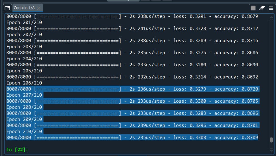
classifier.fit(X_train, y_train, batch_size = 10, epochs = 210)
#Part 3 - Making the predictions and evaluating the model
#Predicting the Test set results
y_pred = classifier.predict(X_test)
y_pred = (y_pred > 0.5)
#Making the Confusion Matrix
from sklearn.metrics import confusion_matrix
cm = confusion_matrix(y_test, y_pred)
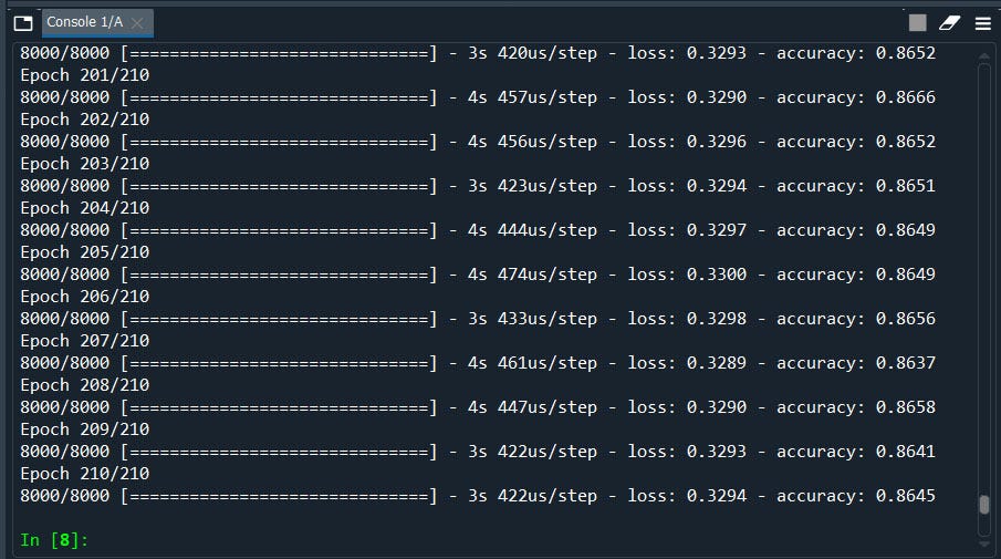
Nice! we have improved our model from 83% to 86%
2.) Next we will use Grid Search to find the best optimizer
Optimizer in brief: optimizer are the algorithms or the methods that is used to calculate weights in order to reduce the losses. I guess you have already heard of Stochastic Gradient Descent and how it works. In layman’s term weights are the optimal values(calculations) that has low loss, in turn high accuracy.
The syntax is almost similar only we need a few modifications
#Function to create model, required for KerasClassifier
def create_model(optimizer='adam'):
model=Sequential()
model.add(Dense(units = 6, kernel_initializer='uniform',activation = 'relu',input_dim = 11))
model.add(Dense(units = 6, kernel_initializer='uniform',activation = 'relu'))
model.add(Dense(units = 1, kernel_initializer = 'uniform', activation = 'sigmoid'))
#compile model
model.compile(optimizer = optimizer,loss = 'binary_crossentropy', metrics = ['accuracy'])
return model
#######################################################
#define the grid search parameters
optimizer = ['SGD', 'RMSprop', 'Adagrad', 'Adadelta', 'Adam', 'Adamax', 'Nadam']
param_grid = dict(optimizer=optimizer)
grid = GridSearchCV(estimator=model, param_grid=param_grid, cv=3)
grid_result = grid.fit(X_train, y_train)
Done! Let’s put all of the pieces together, run the code and see what we got!
# Use scikit-learn to grid search the optimizer
import numpy
from sklearn.model_selection import GridSearchCV
from keras.models import Sequential
from keras.layers import Dense
from keras.wrappers.scikit_learn import KerasClassifier
# Function to create model, required for KerasClassifier
def create_model(optimizer='adam'):
    model=Sequential()
    model.add(Dense(units = 6, kernel_initializer='uniform',activation = 'relu',input_dim = 11))
    model.add(Dense(units = 6, kernel_initializer='uniform',activation = 'relu'))
    model.add(Dense(units = 1, kernel_initializer = 'uniform', activation = 'sigmoid'))
    #compile model
    model.compile(optimizer = optimizer,loss = 'binary_crossentropy', metrics = ['accuracy'])

    return model
#Importing the libraries
import numpy as np
import matplotlib.pyplot as plt
import pandas as pd
#Importing the dataset
dataset = pd.read_csv('Churn_Modelling.csv')
X = dataset.iloc[:, 3:13].values
y = dataset.iloc[:, 13].values
#Encoding categorical data
from sklearn.preprocessing import LabelEncoder, OneHotEncoder
from sklearn.compose import ColumnTransformer
#country column
ct = ColumnTransformer([("Country", OneHotEncoder(), [1])], remainder = 'passthrough')
X = ct.fit_transform(X)
#to avoid dummy variable trap
X = X[:, 1:]
#Male/Female
labelencoder_X = LabelEncoder()
X[:, 3] = labelencoder_X.fit_transform(X[:, 3])
#Splitting the dataset into the Training set and Test set
from sklearn.model_selection import train_test_split
X_train, X_test, y_train, y_test = train_test_split(X, y, test_size = 0.2, random_state = 0)
#Feature Scaling
from sklearn.preprocessing import StandardScaler
sc = StandardScaler()
X_train = sc.fit_transform(X_train)
X_test = sc.transform(X_test)
#############################################################
#create model
model = KerasClassifier(build_fn=create_model, epochs=200, batch_size=10, verbose=1)
#define the grid search parameters
optimizer = ['SGD', 'RMSprop', 'Adagrad', 'Adadelta', 'Adam', 'Adamax', 'Nadam']
param_grid = dict(optimizer=optimizer)
grid = GridSearchCV(estimator=model, param_grid=param_grid, cv=3)
grid_result = grid.fit(X_train, y_train)
#summarize results
print("Best: %f using %s" % (grid_result.best_score_, grid_result.best_params_))
means = grid_result.cv_results_['mean_test_score']
stds = grid_result.cv_results_['std_test_score']
params = grid_result.cv_results_['params']
for mean, stdev, param in zip(means, stds, params):
    print("%f (%f) with: %r" % (mean, stdev, param))
We will have Output Best results as optimizer = SGD ~ Stochastic Gradient Descent.
The results may vary depending on seed value as well as cross-validation cv value. It takes time to get the output. Therefore I decided to write the output from my records rather than using a screenshot.
Now let’s use the optimizer as ‘SGD’ and see how much it improves. Generally ‘adam’ is the commonly used but believed to be optimized version of all. But in a few cases, another optimizer outperforms ‘adam’ such as this one.
#Importing the libraries
import numpy as np
import matplotlib.pyplot as plt
import pandas as pd
#Importing the dataset
dataset = pd.read_csv('Churn_Modelling.csv')
X = dataset.iloc[:, 3:13].values
y = dataset.iloc[:, 13].values
#Encoding categorical data
from sklearn.preprocessing import LabelEncoder, OneHotEncoder
from sklearn.compose import ColumnTransformer
#country column
ct = ColumnTransformer([("Country", OneHotEncoder(), [1])], remainder = 'passthrough')
X = ct.fit_transform(X)
#to avoid dummy variable trap
X = X[:, 1:]
#Male/Female
labelencoder_X = LabelEncoder()
X[:, 3] = labelencoder_X.fit_transform(X[:, 3])
#Splitting the dataset into the Training set and Test set
from sklearn.model_selection import train_test_split
X_train, X_test, y_train, y_test = train_test_split(X, y, test_size = 0.2, random_state = 0)
#Feature Scaling
from sklearn.preprocessing import StandardScaler
sc = StandardScaler()
X_train = sc.fit_transform(X_train)
X_test = sc.transform(X_test)
#Importing the Keras libraries and packages
import keras
from keras.models import Sequential
from keras.layers import Dense
#Initialising the ANN
classifier = Sequential()
#Adding the input layer and the first hidden layer
classifier.add(Dense(units = 6, kernel_initializer = 'uniform', activation = 'relu', input_dim = 11))
#Adding the second hidden layer
classifier.add(Dense(units = 6, kernel_initializer = 'uniform', activation = 'relu'))
# Adding the output layer
classifier.add(Dense(units = 1, kernel_initializer = 'uniform', activation = 'sigmoid'))
#Compiling the ANN
classifier.compile(optimizer = 'SGD', loss = 'binary_crossentropy', metrics = ['accuracy'])
#Fitting the ANN to the Training set
classifier.fit(X_train, y_train, batch_size = 10, epochs = 100)
#Part 3 - Making the predictions and evaluating the model
#Predicting the Test set results
y_pred = classifier.predict(X_test)
y_pred = (y_pred > 0.5)
#Making the Confusion Matrix
from sklearn.metrics import confusion_matrix
cm = confusion_matrix(y_test, y_pred)
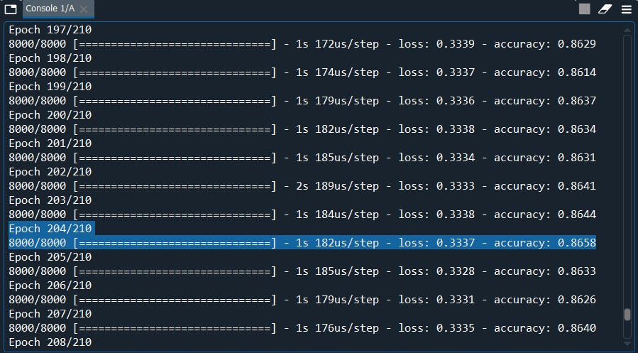
Well, we have slightly improved our model with the SGD optimizer early at the 204 epoch, probably because of my seed number.
Next, we have the Learning rate and the momentum.
3.) Learning Rate and momentum
Learning rate in brief: The amount of rate that the weights are updated during training is referred as the step size or the “learning rate.” Learning rate measures how much the current situation affects the next step, while momentum measures how much past steps affect the next step.
In simple words, it’s the number of steps that will be used to calculate the weights.
We will use the same template with a few modifications to get the best learning rate and momentum.
def create_model(learn_rate=0.01, momentum=0):
model=Sequential()
model.add(Dense(units = 6, kernel_initializer='uniform',activation = 'relu',input_dim = 11))
model.add(Dense(units = 6, kernel_initializer='uniform',activation = 'relu'))
model.add(Dense(units = 1, kernel_initializer = 'uniform', activation = 'sigmoid'))
optimizer = SGD(lr=0.01,momentum = momentum)
#compile model
model.compile(optimizer = optimizer,loss = 'binary_crossentropy', metrics = ['accuracy'])
return model
##############################################3
#define the grid search parameters
learn_rate = [0.001, 0.01, 0.1, 0.2, 0.3]
momentum = [0.0, 0.2, 0.4, 0.6, 0.8, 0.9]
param_grid = dict(learn_rate=learn_rate, momentum=momentum)
grid = GridSearchCV(estimator=model, param_grid=param_grid, cv=3)
Let’s put all of this together and see what we got.
#Use scikit-learn to grid search the learning rate and momentum
import numpy
from sklearn.model_selection import GridSearchCV
from keras.models import Sequential
from keras.layers import Dense
from keras.wrappers.scikit_learn import KerasClassifier
from keras.optimizers import SGD
#Function to create model, required for KerasClassifier
def create_model(learn_rate=0.01, momentum=0):
model=Sequential()
model.add(Dense(units = 6, kernel_initializer='uniform',activation = 'relu',input_dim = 11))
model.add(Dense(units = 6, kernel_initializer='uniform',activation = 'relu'))
model.add(Dense(units = 1, kernel_initializer = 'uniform', activation = 'sigmoid'))
optimizer = SGD(lr=0.01,momentum = momentum)
#compile model
model.compile(optimizer = optimizer,loss = 'binary_crossentropy', metrics = ['accuracy'])
return model
#Importing the libraries
import numpy as np
import matplotlib.pyplot as plt
import pandas as pd
#Importing the dataset
dataset = pd.read_csv('Churn_Modelling.csv')
X = dataset.iloc[:, 3:13].values
y = dataset.iloc[:, 13].values
#Encoding categorical data
from sklearn.preprocessing import LabelEncoder, OneHotEncoder
from sklearn.compose import ColumnTransformer
#country column
ct = ColumnTransformer([("Country", OneHotEncoder(), [1])], remainder = 'passthrough')
X = ct.fit_transform(X)
#to avoid dummy variable trap
X = X[:, 1:]
#Male/Female
labelencoder_X = LabelEncoder()
X[:, 3] = labelencoder_X.fit_transform(X[:, 3])
#Splitting the dataset into the Training set and Test set
from sklearn.model_selection import train_test_split
X_train, X_test, y_train, y_test = train_test_split(X, y, test_size = 0.2, random_state = 0)
#Feature Scaling
from sklearn.preprocessing import StandardScaler
sc = StandardScaler()
X_train = sc.fit_transform(X_train)
X_test = sc.transform(X_test)
#################################################
#create model
model = KerasClassifier(build_fn=create_model, epochs=210, batch_size=10, verbose=1)
#define the grid search parameters
learn_rate = [0.001, 0.01, 0.1, 0.2, 0.3]
momentum = [0.0, 0.2, 0.4, 0.6, 0.8, 0.9]
param_grid = dict(learn_rate=learn_rate, momentum=momentum)
grid = GridSearchCV(estimator=model, param_grid=param_grid, cv=3)
grid_result = grid.fit(X_train, y_train)
#summarize results
print("Best: %f using %s" % (grid_result.best_score_, grid_result.best_params_))
means = grid_result.cv_results_['mean_test_score']
stds = grid_result.cv_results_['std_test_score']
params = grid_result.cv_results_['params']
for mean, stdev, param in zip(means, stds, params):
print("%f (%f) with: %r" % (mean, stdev, param))
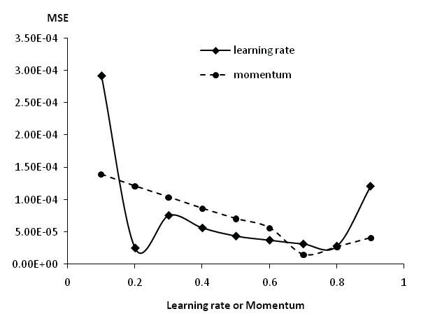
We will have an output of the Best learning rate of 0.01 and a momentum of 0.5
Now we can use these learning rates and momentum in our optimizer to improve our accuracy score.
Next, we will move on to Kernel initializer.
4.) Kernel Initializer
Kernel initializer is a fancy term for which statistical distribution or function to use for initialising the weights.
As usual, we only need a few modifications for the kernel initializer
#Function to create model, required for KerasClassifier
def create_model(init_mode='uniform'):
model=Sequential()
model.add(Dense(units = 6, kernel_initializer= init_mode, activation = 'relu',input_dim = 11))
model.add(Dense(units = 6, kernel_initializer='uniform',activation = 'relu'))
model.add(Dense(units = 1, kernel_initializer = 'uniform', activation = 'sigmoid'))
#compile model
model.compile(optimizer = 'SGD',loss = 'binary_crossentropy', metrics = ['accuracy'])
return model
############################################
#create model
model = KerasClassifier(build_fn=create_model, epochs=210, batch_size=10, verbose=1)
#define the grid search parameters
init_mode = ['uniform', 'lecun_uniform', 'normal', 'zero', 'glorot_normal', 'glorot_uniform', 'he_normal', 'he_uniform']
param_grid = dict(init_mode=init_mode)
grid = GridSearchCV(estimator=model, param_grid=param_grid, cv=3)
grid_result = grid.fit(X_train, y_train)
Done! Let’s put all the pieces together and see which kernel initializer is the best.
#Kernal Initialization
import numpy
from sklearn.model_selection import GridSearchCV
from keras.models import Sequential
from keras.layers import Dense
from keras.wrappers.scikit_learn import KerasClassifier
from keras.optimizers import SGD
#Function to create model, required for KerasClassifier
def create_model(init_mode='uniform'):
model=Sequential()
model.add(Dense(units = 6, kernel_initializer= init_mode, activation = 'relu',input_dim = 11))
model.add(Dense(units = 6, kernel_initializer='uniform',activation = 'relu'))
model.add(Dense(units = 1, kernel_initializer = 'uniform', activation = 'sigmoid'))
#compile model
model.compile(optimizer = 'SGD',loss = 'binary_crossentropy', metrics = ['accuracy'])
return model
#Importing the libraries
import numpy as np
import matplotlib.pyplot as plt
import pandas as pd
#Importing the dataset
dataset = pd.read_csv('Churn_Modelling.csv')
X = dataset.iloc[:, 3:13].values
y = dataset.iloc[:, 13].values
#Encoding categorical data
from sklearn.preprocessing import LabelEncoder, OneHotEncoder
from sklearn.compose import ColumnTransformer
#country column
ct = ColumnTransformer([("Country", OneHotEncoder(), [1])], remainder = 'passthrough')
X = ct.fit_transform(X)
#to avoid dummy variable trap
X = X[:, 1:]
#Male/Female
labelencoder_X = LabelEncoder()
X[:, 3] = labelencoder_X.fit_transform(X[:, 3])
#Splitting the dataset into the Training set and Test set
from sklearn.model_selection import train_test_split
X_train, X_test, y_train, y_test = train_test_split(X, y, test_size = 0.2, random_state = 0)
#Feature Scaling
from sklearn.preprocessing import StandardScaler
sc = StandardScaler()
X_train = sc.fit_transform(X_train)
X_test = sc.transform(X_test)
############################################
#create model
model = KerasClassifier(build_fn=create_model, epochs=210, batch_size=10, verbose=1)
#define the grid search parameters
init_mode = ['uniform', 'lecun_uniform', 'normal', 'zero', 'glorot_normal', 'glorot_uniform', 'he_normal', 'he_uniform']
param_grid = dict(init_mode=init_mode)
grid = GridSearchCV(estimator=model, param_grid=param_grid, cv=3)
grid_result = grid.fit(X_train, y_train)
#summarize results
print("Best: %f using %s" % (grid_result.best_score_, grid_result.best_params_))
means = grid_result.cv_results_['mean_test_score']
stds = grid_result.cv_results_['std_test_score']
params = grid_result.cv_results_['params']
for mean, stdev, param in zip(means, stds, params):
print("%f (%f) with: %r" % (mean, stdev, param))
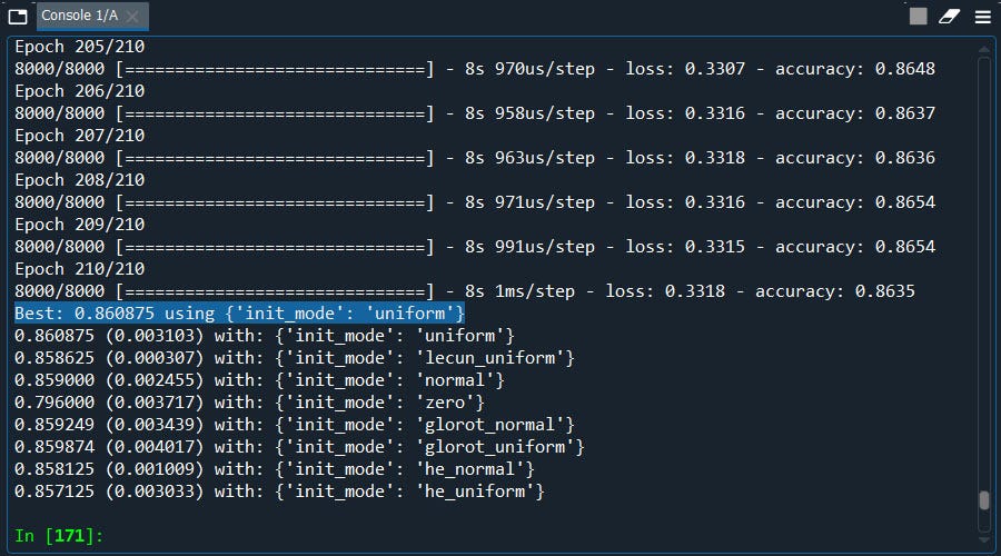
Well, what got here….. The best average score is ‘uniform’ which we are already using.
Next, we have Neuron Activation.
5.) Neuron activation is the parameter where we define the non-linearity function such as relu, sigmoid, leaky relu, softmax. I believe you are already aware of working of those functions. However the would like to mention the rule of thumb for the most commonly used activation functions
Relu is for non-linear data.
Sigmoid is if we want the probability of 0 or 1, Yes or No in classification problem.
Softmax is for when we perform multi-classification.
To perform the Grid Search for neuron activation we will make a few changes as shown below.
def create_model(activation='relu'):
model=Sequential()
model.add(Dense(units = 6, kernel_initializer= 'uniform', activation = activation,input_dim = 11))
model.add(Dense(units = 6, kernel_initializer='uniform',activation = 'relu'))
model.add(Dense(units = 1, kernel_initializer = 'uniform', activation = 'sigmoid'))
#compile model
model.compile(optimizer = 'SGD',loss = 'binary_crossentropy', metrics = ['accuracy'])
return model
###############################################
#define the grid search parameters
activation = ['softmax', 'softplus', 'softsign', 'relu', 'tanh', 'sigmoid', 'hard_sigmoid', 'linear']
param_grid = dict(activation=activation)
grid = GridSearchCV(estimator=model, param_grid=param_grid, cv=3)
grid_result = grid.fit(X_train, y_train)
Done! That’s it….. Let me put all of the pieces together so that you can use them as a template.
#grid search the Nuron activation function
import numpy
from sklearn.model_selection import GridSearchCV
from keras.models import Sequential
from keras.layers import Dense
from keras.wrappers.scikit_learn import KerasClassifier
from keras.optimizers import SGD
#Function to create model, required for KerasClassifier
def create_model(activation='relu'):
    model=Sequential()
    model.add(Dense(units = 6, kernel_initializer= 'uniform', activation = activation,input_dim = 11))
    model.add(Dense(units = 6, kernel_initializer='uniform',activation = 'relu'))
    model.add(Dense(units = 1, kernel_initializer = 'uniform', activation = 'sigmoid'))
    #compile model
    model.compile(optimizer = 'SGD',loss = 'binary_crossentropy', metrics = ['accuracy'])

    return model
#Importing the libraries
import numpy as np
import matplotlib.pyplot as plt
import pandas as pd
#Importing the dataset
dataset = pd.read_csv('Churn_Modelling.csv')
X = dataset.iloc[:, 3:13].values
y = dataset.iloc[:, 13].values
# Encoding categorical data
from sklearn.preprocessing import LabelEncoder, OneHotEncoder
from sklearn.compose import ColumnTransformer
#country column
ct = ColumnTransformer([("Country", OneHotEncoder(), [1])], remainder = 'passthrough')
X = ct.fit_transform(X)
#to avoid dummy variable trap
X = X[:, 1:]
# Male/Female
labelencoder_X = LabelEncoder()
X[:, 3] = labelencoder_X.fit_transform(X[:, 3])
# Splitting the dataset into the Training set and Test set
from sklearn.model_selection import train_test_split
X_train, X_test, y_train, y_test = train_test_split(X, y, test_size = 0.2, random_state = 0)
# Feature Scaling
from sklearn.preprocessing import StandardScaler
sc = StandardScaler()
X_train = sc.fit_transform(X_train)
X_test = sc.transform(X_test)
############################################
# create model
model = KerasClassifier(build_fn=create_model, epochs=210, batch_size=10, verbose=1)
# define the grid search parameters
activation = ['softmax', 'softplus', 'softsign', 'relu', 'tanh', 'sigmoid', 'hard_sigmoid', 'linear']
param_grid = dict(activation=activation)
grid = GridSearchCV(estimator=model, param_grid=param_grid, cv=3)
grid_result = grid.fit(X_train, y_train)
#summarize results
print("Best: %f using %s" % (grid_result.best_score_, grid_result.best_params_))
means = grid_result.cv_results_['mean_test_score']
stds = grid_result.cv_results_['std_test_score']
params = grid_result.cv_results_['params']
for mean, stdev, param in zip(means, stds, params):
    print("%f (%f) with: %r" % (mean, stdev, param))
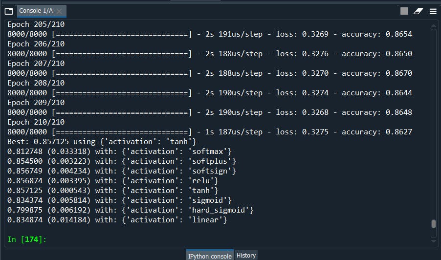
Well, we got the best activation as ‘tanh’ for this example. Now if we put activation as ‘tanh’ it should increase the accuracy.
# Importing the libraries
import numpy as np
import matplotlib.pyplot as plt
import pandas as pd
#Importing the datasetdataset = pd.read_csv('Churn_Modelling.csv')
X = dataset.iloc[:, 3:13].values
y = dataset.iloc[:, 13].values#Encoding categorical data
from sklearn.preprocessing import LabelEncoder, OneHotEncoder
from sklearn.compose import ColumnTransformer
#country column
ct = ColumnTransformer([("Country", OneHotEncoder(), [1])], remainder = 'passthrough')
X = ct.fit_transform(X)
#to avoid dummy variable trap
X = X[:, 1:]
#Male/Female
labelencoder_X = LabelEncoder()
X[:, 3] = labelencoder_X.fit_transform(X[:, 3])
#Splitting the dataset into the Training set and Test set
from sklearn.model_selection import train_test_split
X_train, X_test, y_train, y_test = train_test_split(X, y, test_size = 0.2, random_state = 0)
#Feature Scaling
from sklearn.preprocessing import StandardScaler
sc = StandardScaler()
X_train = sc.fit_transform(X_train)
X_test = sc.transform(X_test)
#Importing the Keras libraries and packages
import keras
from keras.models import Sequential
from keras.layers import Dense
#Initialising the ANN
classifier = Sequential()
#Adding the input layer and the first hidden layer
classifier.add(Dense(units = 6, kernel_initializer = 'uniform', activation = 'tanh', input_dim = 11))
#Adding the second hidden layer
classifier.add(Dense(units = 6, kernel_initializer = 'uniform', activation = 'relu'))
#Adding the output layer
classifier.add(Dense(units = 1, kernel_initializer = 'uniform', activation = 'sigmoid'))
#Compiling the ANN
classifier.compile(optimizer = 'adam', loss = 'binary_crossentropy', metrics = ['accuracy'])
#Fitting the ANN to the Training set
classifier.fit(X_train, y_train, batch_size = 10, epochs = 210)
#Part 3 - Making the predictions and evaluating the model
#Predicting the Test set results
y_pred = classifier.predict(X_test)
y_pred = (y_pred > 0.5)
#Making the Confusion Matrix
from sklearn.metrics import confusion_matrix
cm = confusion_matrix(y_test, y_pred)
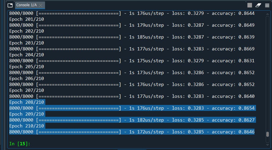
yes, it did by a few decimals.
Next, we have Grid Search for Drop Out Regularization
Drop out is a technique used to prevent a model from overfitting. It is applied between the hidden layers and between the last hidden layer. In simple words the term ‘dropout’ refers to dropping out units (Both hidden and visible) in a neural network
Imagine that if neurons are randomly dropped out of the network during training, that other neurons will have to step in and handle the representation required to make predictions for the missing neurons. This is believed to result in multiple independent internal representations being learned by the network.
The effect is that the network becomes less sensitive to the specific weights of neurons. This in turn results in a network that is capable of better generalization and is less likely to overfit the training data.
Weight constraints also provide an approach to reduce the overfitting of a deep learning neural network model on the training data to improve the performance of the model for new data.
A suite of different vector norms can be used as constraints, provided as classes in the keras.constraints module. They are:
· Maximum norm (max_norm), to force weights to have a magnitude at or below a given limit.
· Non-negative norm (non_neg), to force weights to have a positive magnitude.
· Unit norm (unit_norm), to force weights to have a magnitude of 1.0.
· Min-Max norm (min_max_norm), to force weights to have a magnitude between a range.
Now let's see how can we apply Grid Search for Dropout and Weight Constraints.
from keras.constraints import maxnorm
from keras.layers import Dropout
#Function to create model, required for KerasClassifier
def create_model(dropout_rate=0.0, weight_constraint=0):
model=Sequential()
model.add(Dense(units = 6, kernel_initializer= 'uniform', activation = 'tanh',kernel_constraint=maxnorm(weight_constraint),input_dim = 11))
model.add(Dense(units = 6, kernel_initializer='uniform',activation = 'relu'))
model.add(Dropout(dropout_rate))
model.add(Dense(units = 1, kernel_initializer = 'uniform', activation = 'sigmoid'))
#compile model
model.compile(optimizer = 'SGD',loss = 'binary_crossentropy', metrics = ['accuracy'])
return model
###############################################
#define the grid search parameters
weight_constraint = [1, 2, 3, 4, 5]
dropout_rate = [0.0, 0.1, 0.2, 0.3, 0.4, 0.5, 0.6, 0.7, 0.8, 0.9]
param_grid = dict(dropout_rate=dropout_rate, weight_constraint=weight_constraint)
Alright, the whole code looks the same with a few modifications. let me put all the pieces together so that you can use this as a template
#grid search the Dropout Regularization
import numpy
from sklearn.model_selection import GridSearchCV
from keras.models import Sequential
from keras.layers import Dense
from keras.wrappers.scikit_learn import KerasClassifier
from keras.optimizers import SGD
from keras.constraints import maxnorm
from keras.layers import Dropout
#Function to create model, required for KerasClassifier
def create_model(dropout_rate=0.0, weight_constraint=0):
model=Sequential()
model.add(Dense(units = 6, kernel_initializer= 'uniform', activation = 'tanh',kernel_constraint=maxnorm(weight_constraint),input_dim = 11))
model.add(Dense(units = 6, kernel_initializer='uniform',activation = 'relu'))
model.add(Dropout(dropout_rate))
model.add(Dense(units = 1, kernel_initializer = 'uniform', activation = 'sigmoid'))
#compile model
model.compile(optimizer = 'SGD',loss = 'binary_crossentropy', metrics = ['accuracy'])
return model
#Importing the libraries
import numpy as np
import pandas as pd
#Importing the dataset
dataset = pd.read_csv('Churn_Modelling.csv')
X = dataset.iloc[:, 3:13].values
y = dataset.iloc[:, 13].values
#Encoding categorical data
from sklearn.preprocessing import LabelEncoder, OneHotEncoder
from sklearn.compose import ColumnTransformer
#country column
ct = ColumnTransformer([("Country", OneHotEncoder(), [1])], remainder = 'passthrough')
X = ct.fit_transform(X)
#to avoid dummy variable trap
X = X[:, 1:]
#Male/Female
labelencoder_X = LabelEncoder()
X[:, 3] = labelencoder_X.fit_transform(X[:, 3])
#Splitting the dataset into the Training set and Test set
from sklearn.model_selection import train_test_split
X_train, X_test, y_train, y_test = train_test_split(X, y, test_size = 0.2, random_state = 0)
#Feature Scaling
from sklearn.preprocessing import StandardScaler
sc = StandardScaler()
X_train = sc.fit_transform(X_train)
X_test = sc.transform(X_test)
############################################
#create model
model = KerasClassifier(build_fn=create_model, epochs=210, batch_size=10, verbose=1)
#define the grid search parameters
weight_constraint = [1, 2, 3, 4, 5]
dropout_rate = [0.0, 0.1, 0.2, 0.3, 0.4, 0.5, 0.6, 0.7, 0.8, 0.9]
param_grid = dict(dropout_rate=dropout_rate, weight_constraint=weight_constraint)
grid = GridSearchCV(estimator=model, param_grid=param_grid, cv=3)
grid_result = grid.fit(X_train, y_train)
#summarize results
print("Best: %f using %s" % (grid_result.best_score_, grid_result.best_params_))
means = grid_result.cv_results_['mean_test_score']
stds = grid_result.cv_results_['std_test_score']
params = grid_result.cv_results_['params']
for mean, stdev, param in zip(means, stds, params):
print("%f (%f) with: %r" % (mean, stdev, param))
Finally, we are into the last one Grid Search for the Best Optimal number of neurons.
7.) Grid Search for the Optimal Number of Neurons
As we know neuron takes one or more inputs that are computed by values called “weights” and then passed to a non-linear function which is known as an activation function,
In general the rule of thumb to select the best number of neurons is to take half of the actual input i.e. input dimensions (n/2). However we can also use the grid search feature to find the best optimal number of neurons so that we can improve our model.
#Function to create model, required for KerasClassifier
def create_model(neurons=1):
model=Sequential()
model.add(Dense(units =neurons, kernel_initializer= 'uniform', activation = 'tanh',kernel_constraint=maxnorm(4),input_dim = 11))
model.add(Dense(units = 6, kernel_initializer='uniform',activation = 'relu'))
model.add(Dropout(0.2))
model.add(Dense(units = 1, kernel_initializer = 'uniform', activation = 'sigmoid'))
#compile model
model.compile(optimizer = 'SGD',loss = 'binary_crossentropy', metrics = ['accuracy'])
return model
###########################################
#define the grid search parameters
neurons = [1, 5, 10, 15, 20, 25, 30]
param_grid = dict(neurons=neurons)
grid = GridSearchCV(estimator=model, param_grid=param_grid, cv=3)
grid_result = grid.fit(X_train, y_train)
Let’s put all of these together to use as templates.
#grid search the Dropout Regularization
import numpy
from sklearn.model_selection import GridSearchCV
from keras.models import Sequential
from keras.layers import Dense
from keras.wrappers.scikit_learn import KerasClassifier
from keras.optimizers import SGD
from keras.constraints import maxnorm
from keras.layers import Dropout
# Function to create model, required for KerasClassifier
def create_model(neurons=1):
model=Sequential()
model.add(Dense(units =neurons, kernel_initializer= 'uniform', activation = 'tanh',kernel_constraint=maxnorm(4),input_dim = 11))
model.add(Dense(units = 6, kernel_initializer='uniform',activation = 'relu'))
model.add(Dropout(0.2))
model.add(Dense(units = 1, kernel_initializer = 'uniform', activation = 'sigmoid'))
#compile model
model.compile(optimizer = 'SGD',loss = 'binary_crossentropy', metrics = ['accuracy'])
return model
# Importing the libraries
import numpy as np
import matplotlib.pyplot as plt
import pandas as pd
# Importing the dataset
dataset = pd.read_csv('Churn_Modelling.csv')
X = dataset.iloc[:, 3:13].values
y = dataset.iloc[:, 13].values
# Encoding categorical data
from sklearn.preprocessing import LabelEncoder, OneHotEncoder
from sklearn.compose import ColumnTransformer
#country column
ct = ColumnTransformer([("Country", OneHotEncoder(), [1])], remainder = 'passthrough')
X = ct.fit_transform(X)
#to avoid dummy variable trap
X = X[:, 1:]
# Male/Female
labelencoder_X = LabelEncoder()
X[:, 3] = labelencoder_X.fit_transform(X[:, 3])
# Splitting the dataset into the Training set and Test set
from sklearn.model_selection import train_test_split
X_train, X_test, y_train, y_test = train_test_split(X, y, test_size = 0.2, random_state = 0)
# Feature Scaling
from sklearn.preprocessing import StandardScaler
sc = StandardScaler()
X_train = sc.fit_transform(X_train)
X_test = sc.transform(X_test)
############################################
# create model
model = KerasClassifier(build_fn=create_model, epochs=210, batch_size=10, verbose=1)
# define the grid search parameters
neurons = [1, 5, 10, 15, 20, 25, 30]
param_grid = dict(neurons=neurons)
grid = GridSearchCV(estimator=model, param_grid=param_grid, cv=3)
grid_result = grid.fit(X_train, y_train)
# summarize results
print("Best: %f using %s" % (grid_result.best_score_, grid_result.best_params_))
means = grid_result.cv_results_['mean_test_score']
stds = grid_result.cv_results_['std_test_score']
params = grid_result.cv_results_['params']
for mean, stdev, param in zip(means, stds, params):
print("%f (%f) with: %r" % (mean, stdev, param))
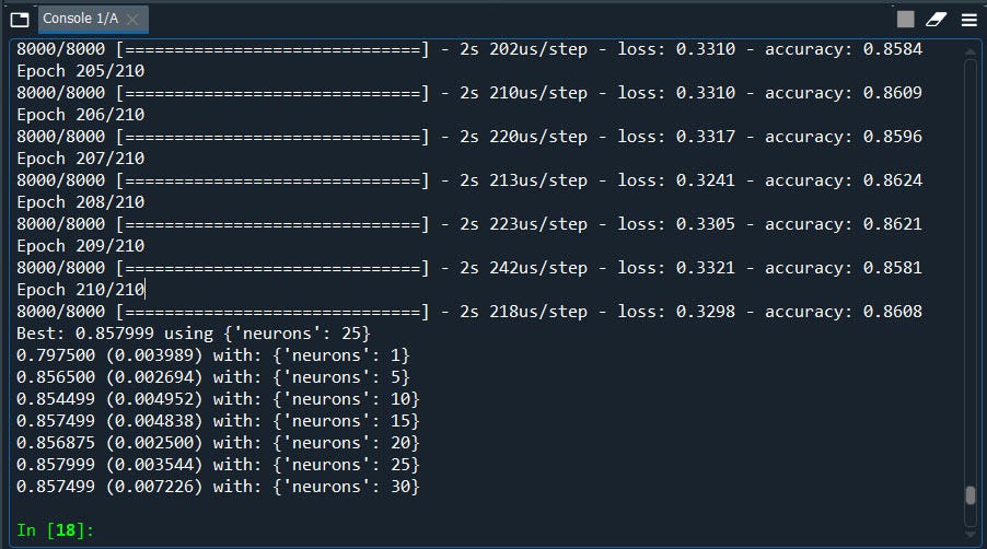
We have our best score: 25 Let’s redo our model with 25 neurons
#Importing the libraries
import numpy as np
import matplotlib.pyplot as plt
import pandas as pd
from keras.constraints import maxnorm
from keras.layers import Dropout
#Importing the dataset
dataset = pd.read_csv('Churn_Modelling.csv')
X = dataset.iloc[:, 3:13].values
y = dataset.iloc[:, 13].values
#Encoding categorical data
from sklearn.preprocessing import LabelEncoder, OneHotEncoder
from sklearn.compose import ColumnTransformer
#country column
ct = ColumnTransformer([("Country", OneHotEncoder(), [1])], remainder = 'passthrough')
X = ct.fit_transform(X)
#to avoid dummy variable trap
X = X[:, 1:]
#Male/Female
labelencoder_X = LabelEncoder()
X[:, 3] = labelencoder_X.fit_transform(X[:, 3])
#Splitting the dataset into the Training set and Test set
from sklearn.model_selection import train_test_split
X_train, X_test, y_train, y_test = train_test_split(X, y, test_size = 0.2, random_state = 0)
# Feature Scaling
from sklearn.preprocessing import StandardScaler
sc = StandardScaler()
X_train = sc.fit_transform(X_train)
X_test = sc.transform(X_test)
# Part 2 - Now let's make the ANN!
# Importing the Keras libraries and packages
import keras
from keras.models import Sequential
from keras.layers import Dense
# Initialising the ANN
classifier = Sequential()
#Adding the input layer and the first hidden layer
classifier.add(Dense(units = 25, kernel_initializer = 'uniform', activation = 'tanh', input_dim = 11))
#Adding the second hidden layer
classifier.add(Dense(units = 6, kernel_initializer = 'uniform', activation = 'relu'))
classifier.add(Dropout(0.2))
#Adding the output layer
classifier.add(Dense(units = 1, kernel_initializer = 'uniform', activation = 'sigmoid'))
#Compiling the ANN
classifier.compile(optimizer = 'adam', loss = 'binary_crossentropy', metrics = ['accuracy'])
#Fitting the ANN to the Training set
classifier.fit(X_train, y_train, batch_size = 10, epochs = 210)
#Part 3 - Making the predictions and evaluating the model
#Predicting the Test set results
y_pred = classifier.predict(X_test)
y_pred = (y_pred > 0.5)
#Making the Confusion Matrix
from sklearn.metrics import confusion_matrix
cm = confusion_matrix(y_test, y_pred)
Nice. again we have improved our model from 86 to 87% and we have still had a lot of room for improvement with a few more tweaks.
Well it’s a long article, i tried my best to keep it as simple as possible keeping all the important concepts intact. I hope you enjoyed and able to use this Grid Search in your day to day deep learning methods.
Some of my alternative internet presences are Facebook, Instagram, Udemy, Blogger, Issuu, and more.
Also available on Quora @ https://www.quora.com/profile/Rupak-Bob-Roy
Have a good day


Comments
Post a Comment