What is PCA and How can we apply Real Quick and Easy Way?
What is PCA and How can we apply Real Quick and Easy Way?
Learn how to apply Principal Component Analysis (PCA) using python

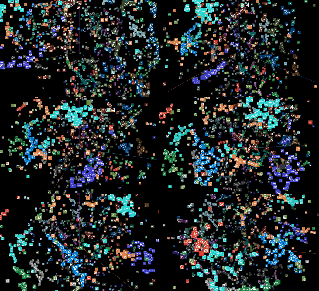
What is Principal Component Analysis (PCA)?
Principal Component Analysis or PCA is a statistical procedure that allows us to summarize/extract the only important data that explains the whole dataset.
Principal component analysis today is one of the most popular multivariate statistical techniques. PCA is the mother method for multivariate data analysis MVDA
It has been widely used in the areas of pattern recognition and signal processing and in statistical analysis to reduce the dimension, in simple words, to understand and extract only the important factors that explain the whole data. This helps in avoiding unnecessary data being processed.
Let’s understand this with the help of an example:
For this example we will use one of the famous available datasets ‘wine_quality’ where we have the key components factors of wine and its customer.
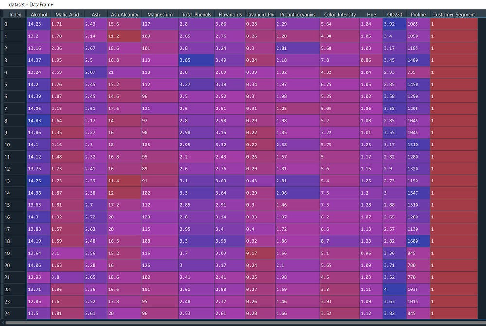
What we will do is with PCA we will try to find out the few key component factors that describe the whole dataset and to validate we will cross-check it with performance metrics.
Let’s get started!
First, we will import the required libraries and import the dataset then define our independent variable X and dependent variable y then split the dataset into train and test.
import numpy as np
import matplotlib.pyplot as plt
import pandas as pd
#Importing the dataset
dataset = pd.read_csv('Wine.csv')
X = dataset.iloc[:, 0:13].values
y = dataset.iloc[:, 13].values
#Splitting the dataset into the Training set and Test set
from sklearn.model_selection import train_test_split
X_train, X_test, y_train, y_test = train_test_split(X, y, test_size = 0.2, random_state = 0)
We will also normalize/scale the data into a common range to reduce the magnitude/spread of data points without losing their original meaning.
#Feature Scaling
from sklearn.preprocessing import StandardScaler
sc = StandardScaler()
X_train = sc.fit_transform(X_train)
X_test = sc.transform(X_test)
Time to apply PCA!
#Applying PCA
from sklearn.decomposition import PCA
pca = PCA(n_components = 3)
X_train = pca.fit_transform(X_train)
X_test = pca.transform(X_test)
N_components refer to give us 3 important components/columns that explain most of the data set.
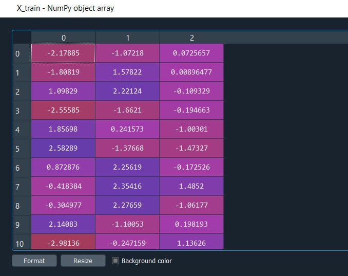
Now the extractions are done from our independent variables X_train and X_test let’s see what we got in our X_train and X_test.
And yes i think you are aware of that we don’t have to write again ‘pca.fit…..’ just simply ‘pca.transform’ will do. Python automatically learns that you are using PCA for this transformation purpose.
Now using this explained_variance we can understand how much each of the 3 principal components is explaining.
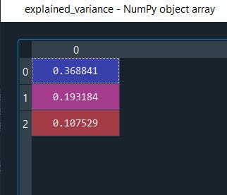
Alright it's 65%
If we want to view how much each variable is explaining the whole dataset just replace n_components = 3 with ‘n_components = None’ and with ‘explained_variance = pca.explained_variance_ratio_’ you will observe the scores of the 3 topmost components are high.
Note: in PCA. The components are sorted with scores from highest to low as you have seen. So it is difficult to identity which components corresponds to a particular column of the dataset. To solve this issue we have an another method call Feature Selection which will learn in next article. Subsribe and Stay Tune!
Thus PCA is very helpful when it comes to analyzing big data where you have 100000 columns and it off-course becomes time-consuming to process all of them and where predictive modelling to predict a future event is more important than just analyzing.
Now its time to fit our data in a model and will check how much accuracy we can derive
# Fitting Logistic Regression to the Training set
from sklearn.linear_model import LogisticRegression
classifier = LogisticRegression(random_state = 0)
classifier.fit(X_train, y_train)
# Predicting the Test set results
y_pred = classifier.predict(X_test)
Here as you can see, we are using logistic regression, random_state is just a seed number to avoid randomness for the set of data for each time the algorithm computes. Then we will predict with unseen data (X_test)
We will use our regular confusion matrix then the accuracy score metric.
# Making the Confusion Matrix
from sklearn.metrics import confusion_matrix
cm = confusion_matrix(y_test, y_pred)
#Another evaluation Metrics
print('Accuracy Score:', metrics.accuracy_score(y_test, y_pred))
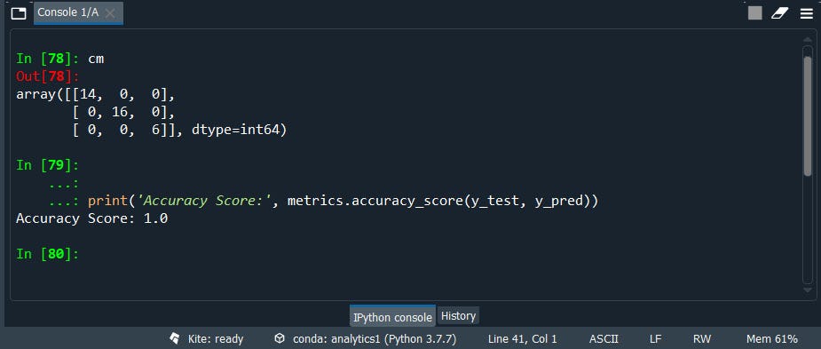
Wowwww we have a 100% accuracy score even in the confusion matrix(cm) is able to predict class perfectly to our test dataset(unseen data).
Let’s redo with 5 n_components and see if we can take more components.
#Splitting the dataset into the Training set and Test set
from sklearn.model_selection import train_test_split
X_train, X_test, y_train, y_test = train_test_split(X, y, test_size = 0.2, random_state = 0)
#Feature Scaling
from sklearn.preprocessing import StandardScaler
sc = StandardScaler()
X_train = sc.fit_transform(X_train)
X_test = sc.transform(X_test)
#Applying PCA
from sklearn.decomposition import PCA
pca = PCA(n_components = 5)
X_train = pca.fit_transform(X_train)
X_test = pca.transform(X_test)
explained_variance = pca.explained_variance_ratio_
#Fitting Logistic Regression to the Training set
from sklearn.linear_model import LogisticRegression
classifier = LogisticRegression(random_state = 0)
classifier.fit(X_train, y_train)
#Predicting the Test set results
y_pred = classifier.predict(X_test)
#Making the Confusion Matrix
from sklearn.metrics import confusion_matrix
cm = confusion_matrix(y_test, y_pred)
#Another evaluation Metrics
from sklearn import metrics
print('Accuracy Score:', metrics.accuracy_score(y_test, y_pred))
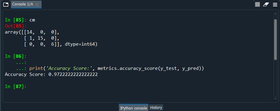
Well, the performance got deteriorate to 97% So the 3 n_components before explains 100% of the dataset. Therefore we can use those 3 n_components from 13 components(columns) to make a predicted model with 100% accuracy.
Now think of this having more than 10000 columns and we are able to extract only a few principal components that explain the whole dataset.
Just imagine how helpful PCA Principal Components Analysis it will be.
Let’s put all of the pieces together.
#Importing the libraries
import numpy as np
import matplotlib.pyplot as plt
import pandas as pd
#Importing the dataset
dataset = pd.read_csv('Wine.csv')
X = dataset.iloc[:, 0:13].values
y = dataset.iloc[:, 13].values
#Splitting the dataset into the Training set and Test set
from sklearn.model_selection import train_test_split
X_train, X_test, y_train, y_test = train_test_split(X, y, test_size = 0.2, random_state = 0)
#Feature Scaling
from sklearn.preprocessing import StandardScaler
sc = StandardScaler()
X_train = sc.fit_transform(X_train)
X_test = sc.transform(X_test)
#Applying PCA
from sklearn.decomposition import PCA
pca = PCA(n_components = 3)
X_train = pca.fit_transform(X_train)
X_test = pca.transform(X_test)
explained_variance = pca.explained_variance_ratio_
#Fitting Logistic Regression to the Training set
from sklearn.linear_model import LogisticRegression
classifier = LogisticRegression(random_state = 0)
classifier.fit(X_train, y_train)
#Predicting the Test set results
y_pred = classifier.predict(X_test)
#Making the Confusion Matrix
from sklearn.metrics import confusion_matrix
cm = confusion_matrix(y_test, y_pred)
#Another evaluation Metrics
print('Accuracy Score:', metrics.accuracy_score(y_test, y_pred))
#---------------------------------------------------------------
#Let's redo and check the accuracy of our model with 5 components
#Splitting the dataset into the Training set and Test set
from sklearn.model_selection import train_test_split
X_train, X_test, y_train, y_test = train_test_split(X, y, test_size = 0.2, random_state = 0)
#Feature Scaling
from sklearn.preprocessing import StandardScaler
sc = StandardScaler()
X_train = sc.fit_transform(X_train)
X_test = sc.transform(X_test)
#Applying PCA
from sklearn.decomposition import PCA
pca = PCA(n_components = 5)
X_train = pca.fit_transform(X_train)
X_test = pca.transform(X_test)
explained_variance = pca.explained_variance_ratio_
#Fitting Logistic Regression to the Training set
from sklearn.linear_model import LogisticRegression
classifier = LogisticRegression(random_state = 0)
classifier.fit(X_train, y_train)
#Predicting the Test set results
y_pred = classifier.predict(X_test)
#Making the Confusion Matrix
from sklearn.metrics import confusion_matrix
cm = confusion_matrix(y_test, y_pred)
#Another evaluation Metrics
from sklearn import metrics
print('Accuracy Score:', metrics.accuracy_score(y_test, y_pred))
Now for those who wish to perform PCA with R programming, i have a whole new course to perform various types of PCA. PCA with Big Data, PCA with Random Forest further divided into classification and regression, PCA with Generalized Boosted Models(GBM), PCA with Generalized Linear Models(GLMNET), PCA with Ensemble, PCA with fscaret, and more.
Did you observe the PCA we just did was UNSUPERVISED? Ya it is
Next will see another type of PCA, Linear Discriminant Analysis (LDA) a Supervised PCA
Thanks for your time to read to the end. I tried my best to keep it short and simple keeping in mind to use this code in our daily life.
I hope you enjoyed it.
Feel Free to ask because “Curiosity Leads To Perfection”
Some of my alternative internet presences are Facebook, Instagram, Udemy, Blogger, Issuu, and more.
Also available on Quora @ https://www.quora.com/profile/Rupak-Bob-Roy
Stay tuned for more updates.! have a good day….
~ Be Happy and Enjoy!

Comments
Post a Comment