Reinforcement Learning | In 31 Steps -using Upper Confidence Bound(UCB) & Thompson Sampling for Social Media Marketing Campaign Click Through Rate Optimization(using Python & R)
using Upper Confidence Bound(UCB) & Thompson Sampling for Social Media Marketing Campaign Click Through Rate Optimization(using Python & R)
Upper Confidence Bound
Upper Confidence Bound (UCB) is one of the advanced methods to perform Reinforcement Learning.
And What is Reinforcement learning? Reinforcement learning is a type of machine learning that enables an agent to learn in an interactive environment by trial and error using feedback from its own actions and experiences.
Let’s take an example.

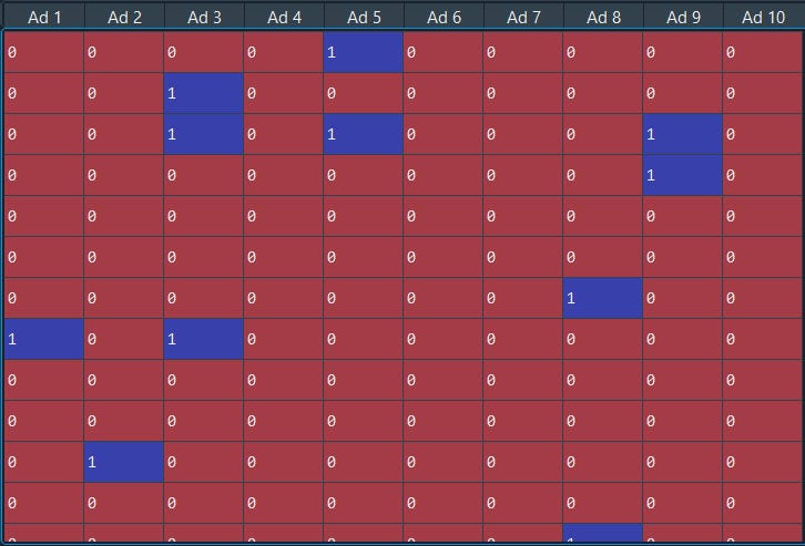
The above data are the 10 versions/types of a social media ad campaign and if the user clicked label as 1 else 0
From the above social ad Campaign, we are not certain which one is performing better or deriving traffic.
We wish to find which is the best ad that works the best i.e. maximize our returns.
One way we can do that is by knowing the distribution. And we can have the distribution of data like people have clicked “ad” or “not” after clicking 1000s 1000s 1000s of times “ad”.
One alternative way to approach this is to do the A/B test on 100 ads or multiple A/B tests and wait until you have a large enough sample and conclude which was is better
The problem here you will have is you will be spending a lot of time and money on the A/B test. They are purely based on exploration and not exploiting the best option, even if you are exploring the best option you will also be exploring the non-optimal option.
Thus A/B tests are only best for exploration.
So UCB is an appropriate and quicker way to explore the best from the rest!’
Let’s import the essential libraries
# Importing the libraries
import numpy as np
import matplotlib.pyplot as plt
import pandas as pd
# Importing the dataset
dataset = pd.read_csv('ads_data.csv')
THE UCB algorithm — the way algorithm works is by rewarding the add version for each round the user clicked.
# Implementing UCB
import math
N = 10000  #number of rows i.e. number of rounds
d = 10
ads_selected = []
numbers_of_selections = [0] * d
sums_of_rewards = [0] * d
total_reward = 0
Here we will define the number of rounds/rows/data (N) we have of the campaign then d = 10 refers to the number of ad versions we have in the campaign
Next, we will create a loop to calculate for all the rounds and the versions of the ad.
for n in range(0, N):
ad = 0
max_upper_bound = 0
for i in range(0, d):
if (numbers_of_selections[i] > 0):
average_reward = sums_of_rewards[i] / numbers_of_selections[i]
delta_i = math.sqrt(3/2 * math.log(n + 1) / numbers_of_selections[i])
upper_bound = average_reward + delta_i
else:
upper_bound = 1e400
if upper_bound > max_upper_bound:
max_upper_bound = upper_bound
ad = i
ads_selected.append(ad)
numbers_of_selections[ad] = numbers_of_selections[ad] + 1
reward = dataset.values[n, ad]
sums_of_rewards[ad] = sums_of_rewards[ad] + reward
total_reward = total_reward + reward
That’s it….our results are stored in the ads_selected object and if we open the ads_selected object we will see for each round (denoted as index) selected the predicted ad version.
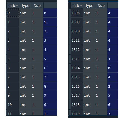
First-round the algorithm selected 1st ad version then when we go down and down to the last round we will see more of 4th ad version is selected.
See algorithm is learning itself the best option by rewarding each ad version in each round.
So now we can easily say that ad version number 4 is better than others with the highest conversion rate.
Finally, it’s the fun part ..visualization.
#Visualizing the results
plt.hist(ads_selected)
plt.title('Histogram of the best Ad ')
plt.xlabel('Social Media Ads')
plt.ylabel('Number of times each ad was selected')
plt.show()
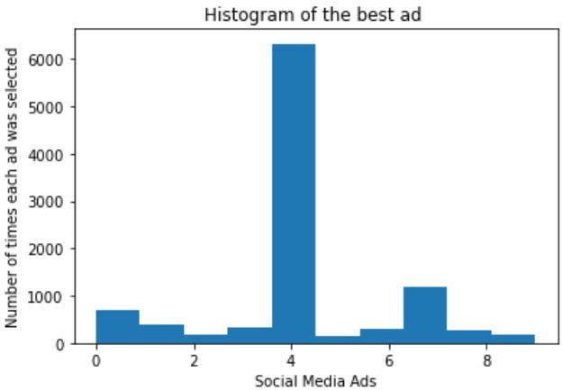
And we can see it’s the 4th ad version is the best optimal option of ad version to use for the marketing campaign.
Let’s put all of this together
# Upper Confidence Bound
# Importing the libraries
import numpy as np
import matplotlib.pyplot as plt
import pandas as pd
# Importing the dataset
dataset = pd.read_csv('ads_data.csv')
# Implementing UCB
import math
N = 10000  #number of rows i.e. number of rounds
d = 10
ads_selected = []
numbers_of_selections = [0] * d
sums_of_rewards = [0] * d
total_reward = 0
for n in range(0, N):
    ad = 0
    max_upper_bound = 0
    for i in range(0, d):
        if (numbers_of_selections[i] > 0):
            average_reward = sums_of_rewards[i] / numbers_of_selections[i]
            delta_i = math.sqrt(3/2 * math.log(n + 1) / numbers_of_selections[i])
            upper_bound = average_reward + delta_i
        else:
            upper_bound = 1e400
        if upper_bound > max_upper_bound:
            max_upper_bound = upper_bound
            ad = i
    ads_selected.append(ad)
    numbers_of_selections[ad] = numbers_of_selections[ad] + 1
    reward = dataset.values[n, ad]
    sums_of_rewards[ad] = sums_of_rewards[ad] + reward
    total_reward = total_reward + reward
#Visualizing the results
plt.hist(ads_selected)
plt.title('Histogram of the best ad ')
plt.xlabel('Social Media Ads')
plt.ylabel('Number of times each ad was selected')
plt.show()
For those who wish to do the same with R, don't worry I got you covered!

# Importing the dataset
dataset = read.csv('ads_data.csv')
#Implementing UCB
N = 10000
d = 10
ads_selected = integer(0)
numbers_of_selections = integer(d)
sums_of_rewards = integer(d)
total_reward = 0
for (n in 1:N) {
  ad = 0
  max_upper_bound = 0
  for (i in 1:d) {
    if (numbers_of_selections[i] > 0) {
      average_reward = sums_of_rewards[i] / numbers_of_selections[i]
      delta_i = sqrt(3/2 * log(n) / numbers_of_selections[i])
      upper_bound = average_reward + delta_i
    } else {
        upper_bound = 1e400
    }
    if (upper_bound > max_upper_bound) {
      max_upper_bound = upper_bound
      ad = i
    }
  }
  ads_selected = append(ads_selected, ad)
  numbers_of_selections[ad] = numbers_of_selections[ad] + 1
  reward = dataset[n, ad]
  sums_of_rewards[ad] = sums_of_rewards[ad] + reward
  total_reward = total_reward + reward
}
#Visualizing the results
hist(ads_selected,
     col = 'blue',
     main = 'Histogram of ads selections',
     xlab = 'Ads',
     ylab = 'Number of times each ad was selected')
Next, I have Thompson Sampling another advanced version of UCB reinforcement learning. Stay Tuned see ya!

Thompson Sampling:
UCB will produce results more similar to an A/B test as we have seen above, while Thompson is more optimized for maximizing long-term overall payoff.
That means UCB is very straightforward, we only look at the upper confidence bound value and the algorithm takes which one has the highest value. However, in Thompson sampling is a probabilistic algorithm that is far more appropriate in handling randomness.
UCB requires updates at every round but Thompson sampling we don’t have to update at every round, they can accommodate delayed feedback.
Take an example of social media ads where you have 1000s 1000s of clicks, in UCB you have to update the algorithm each time it gets an update that is computationally expensive. However in Thompson sampling works batch-wise, like when u get 500 clicks to update the algorithm then 1000 clicks update then 5000 click update, and the algorithm works just fine because it's a probabilistic algorithm. That’s one of the advantages of Thompson Sampling.
So the Thompson Sampling is considered to be better than UCB
We will use the same dataset to compare the results with UCB
#Thompson Sampling
#Importing the libraries
import numpy as np
import matplotlib.pyplot as plt
import pandas as pd
#Importing the dataset
dataset = pd.read_csv('ads_data.csv')
# Implementing Thompson Sampling
import random
N = 10000
d = 10
ads_selected = []
numbers_of_rewards_1 = [0] * d
numbers_of_rewards_0 = [0] * d
total_reward = 0
for n in range(0, N):
    ad = 0
    max_random = 0
    for i in range(0, d):
        random_beta = random.betavariate(numbers_of_rewards_1[i] + 1, numbers_of_rewards_0[i] + 1)
        if random_beta > max_random:
            max_random = random_beta
            ad = i
    ads_selected.append(ad)
    reward = dataset.values[n, ad]
    if reward == 1:
        numbers_of_rewards_1[ad] = numbers_of_rewards_1[ad] + 1
    else:
        numbers_of_rewards_0[ad] = numbers_of_rewards_0[ad] + 1
    total_reward = total_reward + reward
Let’s visualize and compare
#Visualizing the results - Histogram
plt.hist(ads_selected)
plt.title('Histogram of best ad')
plt.xlabel('Social Media Ads')
plt.ylabel('Number of times each ad was selected')
plt.show()
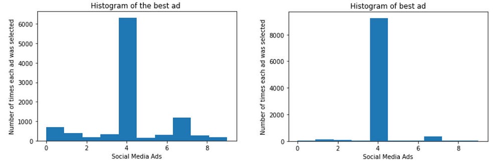
Well we can clearly see the difference in output, with clear evidence Thompson Sampling performs better than UCB.
For those who also wish to perform Thompson Sampling in R, here’s the script.
#Thompson Sampling
#Importing the dataset
dataset = read.csv(file.choose())
#Implementing Thompson Sampling
N = 10000
d = 10
ads_selected = integer(0)
numbers_of_rewards_1 = integer(d)
numbers_of_rewards_0 = integer(d)
total_reward = 0
for (n in 1:N) {
  ad = 0
  max_random = 0
  for (i in 1:d) {
    random_beta = rbeta(n = 1,
                        shape1 = numbers_of_rewards_1[i] + 1,
                        shape2 = numbers_of_rewards_0[i] + 1)
    if (random_beta > max_random) {
      max_random = random_beta
      ad = i
    }
  }
  ads_selected = append(ads_selected, ad)
  reward = dataset[n, ad]
  if (reward == 1) {
    numbers_of_rewards_1[ad] = numbers_of_rewards_1[ad] + 1
  } else {
    numbers_of_rewards_0[ad] = numbers_of_rewards_0[ad] + 1
  }
  total_reward = total_reward + reward
}
#Visualizing the results
hist(ads_selected,
     col = 'blue',
     main = 'Histogram of ads selections',
     xlab = 'Ads',
     ylab = 'Number of times each ad was selected')
Thanks for your time to read to the end. I tried my best to keep it short and simple keeping in mind to use this code in our daily life.
I hope you enjoyed it. Stay tuned for more updates.! have a good day….


Comments
Post a Comment