7 Types of Classification using python

January 23, 2022

7 Types of Classification using python

Full guide to knn, logistic, support vector machine, kernel svm, naive bayes, decision tree classification, random forest classification.

Hi, how are you doing, I hope it's great……….

Today let's understand and perform all types of classification and also we will compare each performance for its accurate prediction.

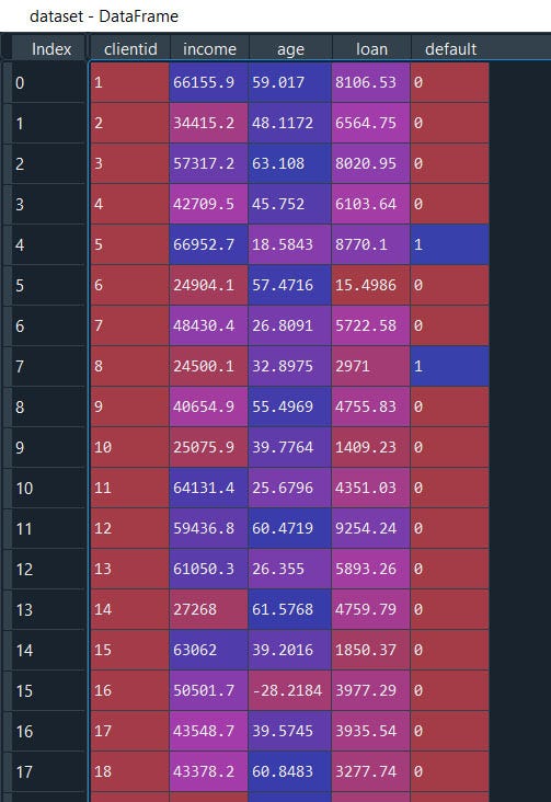
Let’s get started, we will use the demographics to understand and predict if the client will subscribe to a term deposit.

This dataset is public available for research. The details are described in [Moro et al., 2011]. [Moro et al., 2011] S. Moro, R. Laureano and P. Cortez. Using Data Mining for Bank Direct Marketing: An Application of the CRISP-DM Methodology.
In P. Novais et al. (Eds.), Proceedings of the European Simulation and Modelling Conference — ESM’2011, pp. 117–121, Guimarães, Portugal, October, 2011. EUROSIS.

The data is related with direct marketing campaigns of a Portuguese banking institution.
The marketing campaigns were based on phone calls. Often, more than one contact to the same client was required,
in order to access if the product (bank term deposit) would be (or not) subscribed.
The original owners of the dataset:
Created by: Paulo Cortez (Univ. Minho) and Sérgio Moro (ISCTE-IUL) @ 2012

And it contains attributes:

Client ID, Income, Age, Loan, Default

Bank Data set having information about defaulters — Bank Dataset

Let’s get started with our commonly used Classification method:

1.) Logistic Regression then we will use

2.) Knn

3.) Support Vector Machine

4.) Kernel SVM

5.) Naive Bayes

6.) Decision Tree Classification

7.) Random Forest Classification

Any else Classification? Let me know in the comment below.

#Logistic Regression

#Importing the libraries
import numpy as np
import matplotlib.pyplot as plt
import pandas as pd

#Importing the dataset
dataset = pd.read_csv('credit_data.csv', sep=",")

#drop the missing values
dataset = dataset.dropna()

X = dataset.iloc[:,1:4].values
y = dataset.iloc[:, 4].values

Well till here it’s the same as before, load the data then split the data into X and Y where Y is the dependent/target variable 4th column (defaulters column) and rest from 0 to 3 are independent variable X.

Note: in python index position of the columns start from 0 and not from 1.

Then we will split the data into train & test datasets, After we will transform all the column values into one standard value/range that will reduce the spread, magnitude of the data points without losing the original meaning of the data. COOL!

This helps the algorithm to compute the data faster and efficiently.

#Splitting the dataset into the Training set and Test set
from sklearn.model_selection import train_test_split
X_train, X_test, y_train, y_test = train_test_split(X, y, test_size = 0.25, random_state = 0)

from sklearn.preprocessing import StandardScaler
sc = StandardScaler()
X_train = sc.fit_transform(X_train)
X_test = sc.transform(X_test)

Now it's time to fit the data with logistic regression and predict with test results.

#Fitting Logistic Regression to the Training set
from sklearn.linear_model import LogisticRegression
lr_model= LogisticRegression(random_state = 0)
lr_model.fit(X_train, y_train)

# Predicting the Test set results
y_pred = lr_model.predict(X_test)

DONE… !!! super easy isn’t it ?

Let’s compare the predicted results with our original dataset

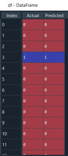
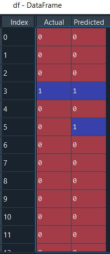
#We can also compare the actual versus predicted
df = pd.DataFrame({'Actual': y_test.flatten(), 'Predicted': y_pred.flatten()})

df

Fatten helps to represent data in a 1-dimensional array like a list.

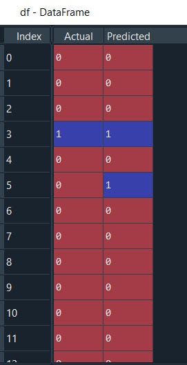
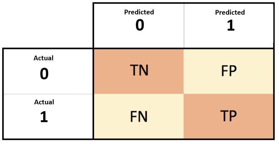
OK. We can see it's quite accurately able to identify. I can understand it's difficult to examine the whole data like this…. For that, we will use aggregated result method ‘confusion matrix’.

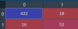
# Making the Confusion Matrix
from sklearn.metrics import confusion_matrix
cm = confusion_matrix(y_test, y_pred)
cm

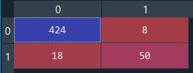
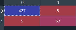
confusion matrix of actual vs predicted for Bank defaulters — Confusion Matrix

NICE.

Confusion Matrix explanation — Confusion Matrix

Our model is able to identify 0’s i.e. non-defaulters which are actually non-defaulters 424 non-defaulters from a total of 500 ( 500 from total 1997 is becoz we have split the dataset into train and test ~ 75% — 25% )

And 18 from 500 are False Negative(FN) which means 18 were defaulters but predicted as non-defaulters. The same goes with 8 from 500 are non-defaulters but predicted as defaulters And prediction 50 refers to defaulters from 500 that are actually defaulters.

This is a really good model with high accuracy and no model is 100% accurate if so THEN there might be some bias issue.

Alright, we have another metric to evaluate the model performance is by using metrics.accuracy_score

#evaluation Metrics
from sklearn import metrics

print('Accuracy Score:', metrics.accuracy_score(y_test, y_pred))
print('Balanced Accuracy Score:', metrics.balanced_accuracy_score(y_test, y_pred))
print('Average Precision:',metrics.average_precision_score(y_test, y_pred))

GREAT! We have a model accuracy score of 0.948 i.e. 95%

And balanced accuracy score of .858 i.e. 86%

And we have one more precision

Precision-Recall is a useful measure of the success of prediction when the classes are very imbalanced. In information retrieval, precision is a measure of result relevancy, while recall is a measure of how many truly relevant results are returned. Precision is more important than recall when you would like to have fewer False Positives in trade-off to have more False Negatives

Finally its time to predict with new input

#if income, age, loan = 66952.7,28,8770.1
import numpy as np 
# Create a numpy array 
new_data = np.array([66952.7,28,8770.1]) 
new_data.dtype
new_data.shape
#We need to reshape to match the dimensions
new_data = new_data.reshape(-1,3)
new_data.shape
#------------------------------------
from sklearn.preprocessing import StandardScaler
sc= StandardScaler()
#scale the data
new_data = sc.fit_transform(new_data)
#We might see the scaled data as 0, 0, 0 but its not its 0.000000e+ and can be view by changing the format
#else inverse transform will give back the original value
inversed = sc.inverse_transform(new_data)
print(inversed)
#-------------------------------------
lr_model.predict(new_data)

#if we wish to enter manually
lr_model.predict([[66952.7,28,8770.1]])

We have an output of array([0], dtype=int64) that is ‘0’ class. Done… we have classified if income, age, loan = 66952.7, 28, 8770.1 seems will be a non-defaulter (class=’0').

BONUS

Save and load the model.

#save the model in the disk
import pickle
# save the model to disk
filename = 'class_model.sav'
pickle.dump(lr_model, open(filename, 'wb'))

# load the model from disk
filename1 = 'class_model.sav'
loaded_model = pickle.load(open(filename1, 'rb'))

#another method using joblib
'''Pickled model as a file using joblib: Joblib is the replacement of pickle as
 it is more efficent on objects that carry large numpy arrays. 
'''

from sklearn.externals import joblib 
  
# Save the model as a pickle in a file 
joblib.dump(lr_model, 'classification.pkl') 
  
# Load the model from the file 
loaded_model2 = joblib.load('classification.pkl')  
  
# Use the loaded model to make predictions 
loaded_model2.predict(X_test)

Let’s put all the pieces together

# Logistic Regression
#Importing the libraries
import numpy as np
import matplotlib.pyplot as plt
import pandas as pd

#Importing the dataset
dataset = pd.read_csv('credit_data.csv', sep=",")

#drop the missing values
dataset = dataset.dropna()

X = dataset.iloc[:,1:4].values
y = dataset.iloc[:, 4].values

#---------------------------------------------------------------
#Splitting the dataset into the Training set and Test set
from sklearn.model_selection import train_test_split
X_train, X_test, y_train, y_test = train_test_split(X, y, test_size = 0.25, random_state = 0)

from sklearn.preprocessing import StandardScaler
sc = StandardScaler()
X_train = sc.fit_transform(X_train)
X_test = sc.transform(X_test)

#Fitting Logistic Regression to the Training set
from sklearn.linear_model import LogisticRegression
lr_model= LogisticRegression(random_state = 0)
lr_model.fit(X_train, y_train)

#Predicting the Test set results
y_pred = lr_model.predict(X_test)

#We can also compare the actual versus predicted
df = pd.DataFrame({'Actual': y_test.flatten(), 'Predicted': y_pred.flatten()})
df

#Making the Confusion Matrix
from sklearn.metrics import confusion_matrix
cm = confusion_matrix(y_test, y_pred)

#evaluation Metrics 
from sklearn import metrics
print('Accuracy Score:', metrics.accuracy_score(y_test, y_pred))  
print('Balanced Accuracy Score:', metrics.balanced_accuracy_score(y_test, y_pred)) 
print('Average Precision:',metrics.average_precision_score(y_test, y_pred))

#if income, age, loan = 66952.7,28,8770.1
import numpy as np 
# Create a numpy array 
new_data = np.array([66952.7,28,8770.1]) 
new_data.dtype
new_data.shape
#We need to reshape to match the dimensions
new_data = new_data.reshape(-1,3)
new_data.shape
#------------------------------------
from sklearn.preprocessing import StandardScaler
sc= StandardScaler()
#scale the data
new_data = sc.fit_transform(new_data)
"""We might see the scaled data as 0, 0, 0 but its not its 0.000000e+ and can be view by changing the format else inverse transform will give back the original value"""

inversed = sc.inverse_transform(new_data)
print(inversed)
#-------------------------------------
lr_model.predict(new_data)

#if we wish to enter manually
lr_model.predict([[66952.7,28,8770.1]])

#---------------------------------------

#save the model in the disk
import pickle
# save the model to disk
filename = 'class_model.sav'
pickle.dump(lr_model, open(filename, 'wb'))

# load the model from disk
filename1 = 'class_model.sav'
loaded_model = pickle.load(open(filename1, 'rb'))

#another method using joblib
'''Pickled model as a file using joblib: Joblib is the replacement of pickle as
 it is more efficent on objects that carry large numpy arrays. 
'''

from sklearn.externals import joblib 
  
# Save the model as a pickle in a file 
joblib.dump(lr_model, 'classification.pkl') 
  
# Load the model from the file 
loaded_model2 = joblib.load('classification.pkl')  
  
# Use the loaded model to make predictions 
loaded_model2.predict(X_test)

Congratulations! We have successfully completed our first Classification model.

Next is KNN

i love travelling — i love traveling, how about you?

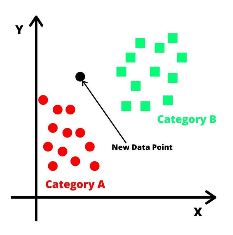
What is KNN?

K-Nearest Neighbors (KNN) is one of the simplest algorithms used in Machine Learning for regression and classification. KNN algorithms classify new data points based on similarity measures (e.g. Euclidean distance function).

Classification is done by a majority vote to its neighbors (K).

K Nearest Neighbors Knn plot — K Nearest Neighbors

Let’s get started on how to apply KNN for classification problems.

#K-Nearest Neighbors (K-NN)

#Importing the libraries
import numpy as np
import matplotlib.pyplot as plt
import pandas as pd

#Importing the dataset
dataset = pd.read_csv('credit_data.csv', sep=",")

#drop the missing values
dataset = dataset.dropna()

X = dataset.iloc[:,1:4].values
y = dataset.iloc[:, 4].values

#-------------------------------------

#Splitting the dataset into the Training set and Test set
from sklearn.model_selection import train_test_split
X_train, X_test, y_train, y_test = train_test_split(X, y, test_size = 0.25, random_state = 0)

from sklearn.preprocessing import StandardScaler
sc = StandardScaler()
X_train = sc.fit_transform(X_train)
X_test = sc.transform(X_test)

Till here it’s the same as before, load the data, define X and Y, split the data, and then scale the independent variables

NOW we will fit the KNN to our training data set where K nearest neighbors K =3 , metric = minkowski which helps to measure three-dimensional Euclidean space and p = 2 is the Power parameter for the Minkowski metric. When p = 1, this is equivalent to using manhattan_distance (l1), and euclidean_distance (l2) for p = 2.

# Fitting K-NN to the Training set

from sklearn.neighbors import KNeighborsClassifier
knn_model = KNeighborsClassifier(n_neighbors = 5, metric = 'minkowski', p = 2)
knn_model.fit(X_train, y_train)

That’s it….!

It's time to predict with the test dataset.

# Predicting the Test set results
y_pred = knn_model.predict(X_test)

Alright let's compare our predicted results with our original results.

#actual versus predicted
df = pd.DataFrame({'Actual': y_test.flatten(), 'Predicted': y_pred.flatten()})

df

Knn actual vs predicted results — KNN Actual Vs Predicted

well it seems,, our model is predicting very good….

Now let’s try to assess our model with evaluation metrics.

First is confusion matrix

# Making the Confusion Matrix

from sklearn.metrics import confusion_matrix
cm = confusion_matrix(y_test, y_pred)

Confusion Matrix of KNN — Confusion Matrix (KNN)

Wow, it's classifying True positive and True negative more accurately than with logistic regression.

#evaluation Metrics 
from sklearn import metrics
print('Accuracy Score:', metrics.accuracy_score(y_test, y_pred))  
print('Balanced Accuracy Score:', metrics.balanced_accuracy_score(y_test, y_pred)) 
print('Average Precision:',metrics.average_precision_score(y_test, y_pred))

WELL WELL WELL

Even the accuracy score is 98% and balanced accuracy score .957 i.e. 96%

And we have one more precision

Precision is more important than recall when you would like to have fewer False Positives in trade-off to have more False Negatives.

Now let's predict with totally unseen random data, if income, age, loan = 66952.7,28,8770.1

#if income, age, loan = 66952.7,28,8770.1

import numpy as np

#Create a numpy array
new_data = np.array([66952.7,28,8770.1])
new_data.dtype
new_data.shape

#We need to reshape to match the dimensions
new_data = new_data.reshape(-1,3)
new_data.shape

#------------------------------------

from sklearn.preprocessing import StandardScaler
sc= StandardScaler()

#scale the data
new_data = sc.fit_transform(new_data)

#We might see the scaled data as 0, 0, 0 but its not its 0.000000e+ and can be view by changing the format

#else inverse transform will give back the original value
inversed = sc.inverse_transform(new_data)
print(inversed)

#-------------------------------------

knn_model.predict(new_data)

#if we wish to enter manually
knn_model.predict([[66952.7,28,8770.1]])

We have an output of array([0], dtype=int64) that is ‘0’ class. Done… we have classified if income, age, loan= 66952.7, 28, 8770.1 seems will to be a non-defaulter (class=’0') with KNN model

Let’s put all of the codes together

#K-Nearest Neighbors (K-NN)

#Importing the libraries
import numpy as np
import matplotlib.pyplot as plt
import pandas as pd

#Importing the dataset
dataset = pd.read_csv('credit_data.csv', sep=",")

#drop the missing values
dataset = dataset.dropna()

X = dataset.iloc[:,1:4].values
y = dataset.iloc[:, 4].values

#------------------------------------------------------
#Splitting the dataset into the Training set and Test set
from sklearn.model_selection import train_test_split
X_train, X_test, y_train, y_test = train_test_split(X, y, test_size = 0.25, random_state = 0)

from sklearn.preprocessing import StandardScaler
sc = StandardScaler()
X_train = sc.fit_transform(X_train)
X_test = sc.transform(X_test)

#Fitting K-NN to the Training set
from sklearn.neighbors import KNeighborsClassifier
knn_model = KNeighborsClassifier(n_neighbors = 5, metric = 'minkowski', p = 2)
knn_model.fit(X_train, y_train)

#Predicting the Test set results
y_pred = knn_model.predict(X_test)

#Model Evaluation------------------------------------
#We can also compare the actual versus predicted
df = pd.DataFrame({'Actual': y_test.flatten(), 'Predicted': y_pred.flatten()})
df

#Making the Confusion Matrix
from sklearn.metrics import confusion_matrix
cm = confusion_matrix(y_test, y_pred)

#evaluation Metrics 
from sklearn import metrics
print('Accuracy Score:', metrics.accuracy_score(y_test, y_pred))  
print('Balanced Accuracy Score:', metrics.balanced_accuracy_score(y_test, y_pred)) 
print('Average Precision:',metrics.average_precision_score(y_test, y_pred))

#---------------------------------------------------

#if income, age, loan = 66952.7,28,8770.1
import numpy as np 
#Create a numpy array 
new_data = np.array([66952.7,28,8770.1]) 
new_data.dtype
new_data.shape
#We need to reshape to match the dimensions
new_data = new_data.reshape(-1,3)
new_data.shape
#------------------------------------
from sklearn.preprocessing import StandardScaler
sc= StandardScaler()
#scale the data
new_data = sc.fit_transform(new_data)
#We might see the scaled data as 0, 0, 0 but its not its 0.000000e+ and can be view by changing the format
#else inverse transform will give back the original value
inversed = sc.inverse_transform(new_data)
print(inversed)
#-------------------------------------
knn_model.predict(new_data)

#if we wish to enter manually
knn_model.predict([[66952.7,28,8770.1]])

#scaled version input data
knn_model.predict([[0.382027,-0.979416,1.45499]])

Congratulations! We have successfully completed our KNN model to classify defaulters

Next is SVM an another powerful classifier

SUPPORT VECTOR MACHINE

What is SVM?

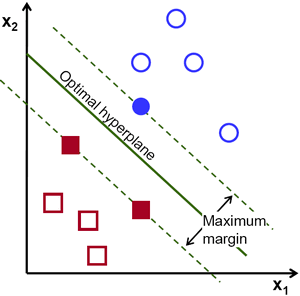
SVM is a supervised machine learning algorithm that can be used for classification or regression problems

In brief, the principle working of SVM is to find the nearest data point(either class) with the help of a hyper-plane. This distance is called as Margin

SVM is highly preferred by many as it produces significant accuracy with less computation power.

Lets get understand this with the help of an example.

#SVM

#Importing the libraries
import numpy as np
import matplotlib.pyplot as plt
import pandas as pd

#Importing the dataset
dataset = pd.read_csv('credit_data.csv', sep=",")

#drop the missing values
dataset = dataset.dropna()
X = dataset.iloc[:,1:4].values
y = dataset.iloc[:, 4].values

#--------------------------------------------
#Splitting the dataset into the Training set and Test set
from sklearn.model_selection import train_test_split
X_train, X_test, y_train, y_test = train_test_split(X, y, test_size = 0.25, random_state = 0)

from sklearn.preprocessing import StandardScaler
sc = StandardScaler()
X_train = sc.fit_transform(X_train)
X_test = sc.transform(X_test)

Well till here it’s the same as others. First, we import the data that defined X & Y, Split the data into train and test sets, scale the independent variables to reduce the magnitude of the spread of data points without losing their original meaning.

It's time to fit the SVM into the training set.

#Fitting SVM to the Training set
from sklearn.svm import SVC
svm_model = SVC(kernel = 'linear', random_state = 0)
svm_model.fit(X_train, y_train)

Now our model is ready to predict with new data

#Predicting the Test set results
y_pred = svm_model.predict(X_test)

Let’s access the performance of our model.

First, we will compare the predicted values with the actual output

#We can also compare the actual versus predicted
df = pd.DataFrame({'Actual': y_test.flatten(), 'Predicted': y_pred.flatten()})

df

SVM Actual vs Predicted Results — Actual Vs Predicted

The second Performance metrics is the Confusion Matrix

# Making the Confusion Matrix

from sklearn.metrics import confusion_matrix
cm = confusion_matrix(y_test, y_pred)

Support Vector Machine Confusion Matrix — Confusion Matrix

It classifies True positive and True negative more accurately than False-positive & False-negative.

Further, we can use scikit sklearn evaluation metrics to assess the model accuracy score.

#evaluation Metrics
from sklearn import metrics
print('Accuracy Score:', metrics.accuracy_score(y_test, y_pred))
print('Balanced Accuracy Score:', metrics.balanced_accuracy_score(y_test, y_pred))
print('Average Precision:',metrics.average_precision_score(y_test, y_pred))

The accuracy score is 95% and the balanced accuracy score is .87 i.e. 87%

And we have one more precision

Precision is more important than recall when you would like to have fewer False Positives in trade-off to have more False Negatives.

Now let's predict with totally unseen random data, if income, age, loan = 66952.7,28,8770.1

#if income, age, loan = 66952.7,28,8770.1

import numpy as np
# Create a numpy array
new_data = np.array([66952.7,28,8770.1])
new_data.dtype
new_data.shape
#We need to reshape to match the dimensions
new_data = new_data.reshape(-1,3)
new_data.shape
#------------------------------------
from sklearn.preprocessing import StandardScaler
sc= StandardScaler()

#scale the data
new_data = sc.fit_transform(new_data)
#We might see the scaled data as 0, 0, 0 but its not its 0.000000e+ and can be view by changing the format

#else inverse transform will give back the original value
inversed = sc.inverse_transform(new_data)
print(inversed)

#---------------------------------------
svm_model.predict(new_data)

#if we wish to enter manually
svm_model.predict([[66952.7,28,8770.1]])

Let’s put all of the codes together.

#SVM

#Importing the libraries

import numpy as np
import matplotlib.pyplot as plt
import pandas as pd

#Importing the dataset
dataset = pd.read_csv('credit_data.csv', sep=",")

#drop the missing values
dataset = dataset.dropna()

X = dataset.iloc[:,1:4].values
y = dataset.iloc[:, 4].values

#-------------------------------------------------------

#Splitting the dataset into the Training set and Test set

from sklearn.model_selection import train_test_split
X_train, X_test, y_train, y_test = train_test_split(X, y, test_size = 0.25, random_state = 0)

from sklearn.preprocessing import StandardScaler
sc = StandardScaler()
X_train = sc.fit_transform(X_train)
X_test = sc.transform(X_test)

#Fitting SVM to the Training set
from sklearn.svm import SVC
svm_model = SVC(kernel = 'linear', random_state = 0)
svm_model.fit(X_train, y_train)

#Predicting the Test set results
y_pred = svm_model.predict(X_test)

#We can also compare the actual versus predicted
df = pd.DataFrame({'Actual': y_test.flatten(), 'Predicted': y_pred.flatten()})

df

#Making the Confusion Matrix

from sklearn.metrics import confusion_matrix
cm = confusion_matrix(y_test, y_pred)

#evaluation Metrics
from sklearn import metrics
print('Accuracy Score:', metrics.accuracy_score(y_test, y_pred))
print('Balanced Accuracy Score:', metrics.balanced_accuracy_score(y_test, y_pred))
print('Average Precision:',metrics.average_precision_score(y_test, y_pred))

#if income, age, loan = 66952.7,28,8770.1
import numpy as np

#Create a numpy array

new_data = np.array([66952.7,28,8770.1])
new_data.dtype
new_data.shape

#We need to reshape to match the dimensions
new_data = new_data.reshape(-1,3)
new_data.shape

#------------------------------------

from sklearn.preprocessing import StandardScaler
sc= StandardScaler()

#scale the data
new_data = sc.fit_transform(new_data)

#We might see the scaled data as 0, 0, 0 but its not its 0.000000e+ and can be view by changing the format

#else inverse transform will give back the original value
inversed = sc.inverse_transform(new_data)
print(inversed)

#-------------------------------------

svm_model.predict(new_data)

#if we wish to enter manually
svm_model.predict([[66952.7,28,8770.1]])

Congratulations! We have successfully completed our SVM model to classify defaulters

Next is Kernel SVM an another powerful SVM

What is Kernel SVM

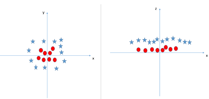
The complexity of Linear SVM grows with the size of the dataset. In simple words Kernel SVM ‘rbf’ transforms complex non-linear data to higher dimensional 3D space to separate the data classes.

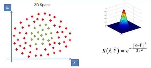
kernel svm helps to transform non-linear data in high dimensional space.

Converting to 3D space. makes it possible to separate the data points

Usually linear and polynomial kernels are less time-consuming and provide less accuracy than the rbf or Gaussian kernels.

So, the rule of thumb is: use linear SVMs (or logistic regression) for linear problems, and nonlinear kernels such as the Radial Basis Function kernel for non-linear problems.

Lets. Compare Linear svm with kernel Radial based svm

# Importing the libraries
import numpy as np
import matplotlib.pyplot as plt
import pandas as pd

# Importing the dataset
dataset = pd.read_csv('credit_data.csv', sep=",")

#drop the missing values
dataset = dataset.dropna()

X = dataset.iloc[:,1:4].values
y = dataset.iloc[:, 4].values

#-----------------------------------------------------------
# Splitting the dataset into the Training set and Test set
from sklearn.model_selection import train_test_split
X_train, X_test, y_train, y_test = train_test_split(X, y, test_size = 0.25, random_state = 0)

#fearure scale
from sklearn.preprocessing import StandardScaler
sc = StandardScaler()
X_train = sc.fit_transform(X_train)
X_test = sc.transform(X_test)

Well till here it’s the same things everywhere. Load the data then define X and Y, split the data, and transform to the standard range to reduce the magnitude of data without losing its original meaning.

Now we will fit the data in both Linear as well as Kernel ‘rbf’ svm to compare both of them.

#Fitting SVM to the Training set
from sklearn.svm import SVC
svm_model = SVC(kernel = 'linear', random_state = 0)
svm_model.fit(X_train, y_train)

#Predicting the Test set results
y_pred = svm_model.predict(X_test)

#Making the Confusion Matrix
from sklearn.metrics import confusion_matrix
cm = confusion_matrix(y_test, y_pred)

#evaluation Metrics 
from sklearn import metrics
print('Accuracy Score:', metrics.accuracy_score(y_test, y_pred))  
print('Balanced Accuracy Score:', metrics.balanced_accuracy_score(y_test, y_pred)) 
print('Average Precision:',metrics.average_precision_score(y_test, y_pred))

#-------------------------------------------------------
#Fitting Kernal SVM to the Training set
from sklearn.svm import SVC
Ksvm_model = SVC(kernel = 'rbf', random_state = 0)
Ksvm_model.fit(X_train, y_train)

#Predicting the Test set results
y_pred = Ksvm_model.predict(X_test)

#Making the Confusion Matrix
from sklearn.metrics import confusion_matrix
cm1 = confusion_matrix(y_test, y_pred)

#evaluation Metrics 
from sklearn import metrics
print('Accuracy Score:', metrics.accuracy_score(y_test, y_pred))  
print('Balanced Accuracy Score:', metrics.balanced_accuracy_score(y_test, y_pred)) 
print('Average Precision:',metrics.average_precision_score(y_test, y_pred))

#Hence we noticed Kernal SVM perform better than SVM

So what we got

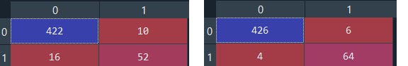
Confusion Matrix: Linear SVM vs Kernal ‘rbf’ SVM — Confusion Matrix: Right | cm | Linear SVM, Left | cm1| Kernel ‘rbf’ SVM

The confusion matrix of Kernel SVM is performing better in identifying True Positive and True Negative than Linear SVM

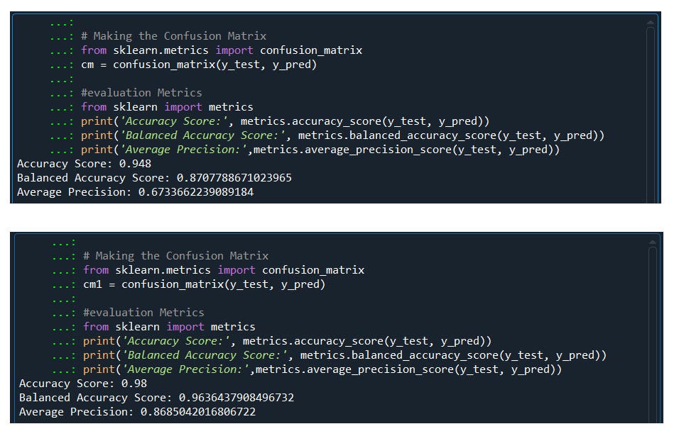
Accuracy score of linear svm and kernal ‘rbf’ svm — Evaluation Metrics | First | Linear SVM, Second | Kernel ‘rbf’ SVM

The accuracy score of our Kernel svm model is better than linear svm

Hence Kernel SVM performs better than Linear SVM.

Finally, with the model, we can predict any new input.

#if income, age, loan = 66952.7,28,8770.1

import numpy as np
#Create a numpy array
new_data = np.array([66952.7,28,8770.1])
new_data.dtype
new_data.shape
#We need to reshape to match the dimensions
new_data = new_data.reshape(-1,3)
new_data.shape

#------------------------------------
from sklearn.preprocessing import StandardScaler
sc= StandardScaler()

#scale the data
new_data = sc.fit_transform(new_data)
#We might see the scaled data as 0, 0, 0 but its not its 0.000000e+ and can be view by changing the format

#else inverse transform will give back the original value
inversed = sc.inverse_transform(new_data)
print(inversed)

#-------------------------------------
Ksvm_model.predict(new_data)

#if we wish to enter manually
Ksvm_model.predict([[66952.7,28,8770.1]])

We have an output of array([0], dtype=int64) that is ‘0’ class. Done… we have classified if income, age, loan = 66952.7, 28, 8770.1 seems will to be a non-defaulter (class=’0') even with Kernel SVM model.

Let’s put all of the codes together.

#Kernal SVM

#Importing the libraries
import numpy as np
import matplotlib.pyplot as plt
import pandas as pd

#Importing the dataset
dataset = pd.read_csv('credit_data.csv', sep=",")

#drop the missing values
dataset = dataset.dropna()

X = dataset.iloc[:,1:4].values
y = dataset.iloc[:, 4].values

#-----------------------------------------------------------
#Splitting the dataset into the Training set and Test set
from sklearn.model_selection import train_test_split
X_train, X_test, y_train, y_test = train_test_split(X, y, test_size = 0.25, random_state = 0)

#fearure scale
from sklearn.preprocessing import StandardScaler
sc = StandardScaler()
X_train = sc.fit_transform(X_train)
X_test = sc.transform(X_test)

#------------------------------------------------------
#Fitting SVM to the Training set
from sklearn.svm import SVC
svm_model = SVC(kernel = 'linear', random_state = 0)
svm_model.fit(X_train, y_train)

#Predicting the Test set results
y_pred = svm_model.predict(X_test)

#Making the Confusion Matrix
from sklearn.metrics import confusion_matrix
cm = confusion_matrix(y_test, y_pred)

#evaluation Metrics 
from sklearn import metrics
print('Accuracy Score:', metrics.accuracy_score(y_test, y_pred))  
print('Balanced Accuracy Score:', metrics.balanced_accuracy_score(y_test, y_pred)) 
print('Average Precision:',metrics.average_precision_score(y_test, y_pred))

#---------------------------------------------------------
# Fitting Kernal SVM to the Training set
from sklearn.svm import SVC
Ksvm_model = SVC(kernel = 'rbf', random_state = 0)
Ksvm_model.fit(X_train, y_train)

#Predicting the Test set results
y_pred = Ksvm_model.predict(X_test)

#Making the Confusion Matrix
from sklearn.metrics import confusion_matrix
cm1 = confusion_matrix(y_test, y_pred)

#evaluation Metrics 
from sklearn import metrics
print('Accuracy Score:', metrics.accuracy_score(y_test, y_pred))  
print('Balanced Accuracy Score:', metrics.balanced_accuracy_score(y_test, y_pred)) 
print('Average Precision:',metrics.average_precision_score(y_test, y_pred))

#Hence we noticed Kernal SVM performs better than SVM

#if income, age, loan = 66952.7,28,8770.1
import numpy as np 
#Create a numpy array 
new_data = np.array([66952.7,28,8770.1]) 
new_data.dtype
new_data.shape
#We need to reshape to match the dimensions
new_data = new_data.reshape(-1,3)
new_data.shape
#------------------------------------
from sklearn.preprocessing import StandardScaler
sc= StandardScaler()
#scale the data
new_data = sc.fit_transform(new_data)
#We might see the scaled data as 0, 0, 0 but its not its 0.000000e+ and can be view by changing the format
#else inverse transform will give back the original value
inversed = sc.inverse_transform(new_data)
print(inversed)
#-------------------------------------
Ksvm_model.predict(new_data)

#if we wish to enter manually
Ksvm_model.predict([[66952.7,28,8770.1]])

Congratulations! We have successfully completed our Kernel SVM model to classify defaulters.

Next is Naive Bayes Classifier.

Introducing Naive Bayes for Classification problems

What is Naive Bayes in short?

Naïve Bayes classifiers are a family of simple “probabilistic classifiers” based on applying Bayes’ theorem.

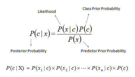
P(c|x) is the posterior probability of class (target) given predictor (attribute).

P(c) is the prior probability of class.
P(x|c) is the likelihood which is the probability of predictor given class.
P(x) is the prior probability of predictor.

Likelihood: How probable is the evidence given that our hypothesis is true.

Prior: How probable was our hypothesis before observing the evidence?

Posterior: How probable is our hypothesis given the observed evidence?

Marginal: How probable is the new evidence under all possible hypotheses?

It's a long chapter about how Naive Bayes works. if are you interested to go in-depth further you can visit my other site. However

In short Naive Bayes uses class of probability method to classify the problem solution.

Let’s see how can we apply Naïve Bayes in classifying the bank defaulters.

#Naive Bayes

#Importing the libraries
import numpy as np
import matplotlib.pyplot as plt
import pandas as pd

#Importing the dataset
dataset = pd.read_csv('credit_data.csv', sep=",")

#drop the missing values
dataset = dataset.dropna()

X = dataset.iloc[:,1:4].values
y = dataset.iloc[:, 4].values

#-----------------------------------------------
#Splitting the dataset into the Training set and Test set
from sklearn.model_selection import train_test_split
X_train, X_test, y_train, y_test = train_test_split(X, y, test_size = 0.25, random_state = 0)

#fearure scaling/Normalization
from sklearn.preprocessing import StandardScaler
sc = StandardScaler()
X_train = sc.fit_transform(X_train)
X_test = sc.transform(X_test)

Alright till here we have the same as above, load the data, define X and Y, split the data into train and test sets then scale the data to reduce the magnitude of the spread of data points without losing their original meaning.

Let’s fit the Naïve Bayes to our data

# Fitting Naive Bayes to the Training set
from sklearn.naive_bayes import GaussianNB
NB_model = GaussianNB()
NB_model.fit(X_train, y_train)

Done,,,, in just 3 lines of code easy isn’t it?

Time to predict on unseen data.

# Predicting the Test set results
y_pred2 = NB_model.predict(X_test)

Done we have our predicted values saved in y_pred2

Now let’s access the model performance with a confusion matrix

# Making the Confusion Matrix
from sklearn.metrics import confusion_matrix
cm2 = confusion_matrix(y_test, y_pred2)

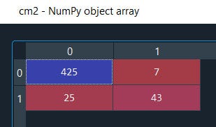
Well, we can see it's classifying True positive and True negative more accurately than False-positive & False-negative.

Further, we can use scikit sklearn evaluation metrics to assess the model accuracy score.

#evaluation Metrics
from sklearn import metrics
print('Accuracy Score:', metrics.accuracy_score(y_test, y_pred))
print('Balanced Accuracy Score:', metrics.balanced_accuracy_score(y_test, y_pred))
print('Average Precision:',metrics.average_precision_score(y_test, y_pred))

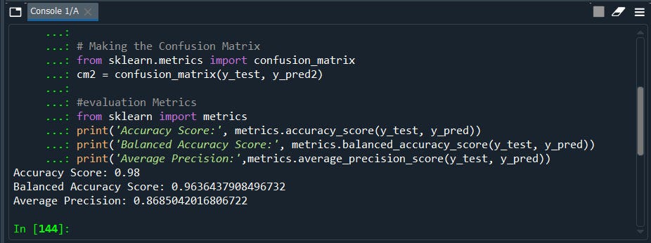
Sk-Learn Evaluation for Naive Bayes — Evaluation Metrics

Well, we got an accuracy score of our model is 98% that’s a good model.

Finally, we can use this model to predict any new data

#if income, age, loan = 66952.7,28,8770.1
import numpy as np 
# Create a numpy array 
new_data = np.array([66952.7,28,8770.1]) 
new_data.dtype
new_data.shape
#We need to reshape to match the dimensions
new_data = new_data.reshape(-1,3)
new_data.shape
#------------------------------------
from sklearn.preprocessing import StandardScaler
sc= StandardScaler()
#scale the data
new_data = sc.fit_transform(new_data)
#We might see the scaled data as 0, 0, 0 but its not its 0.000000e+ and can be view by changing the format
#else inverse transform will give back the original value
inversed = sc.inverse_transform(new_data)
print(inversed)
#-------------------------------------
NB_model.predict(new_data)

#if we wish to enter manually
NB_model.predict([[66952.7,28,8770.1]])

Let’s put all of these codes together.

#Naive Bayes

# Importing the libraries
import numpy as np
import matplotlib.pyplot as plt
import pandas as pd

# Importing the dataset
dataset = pd.read_csv('credit_data.csv', sep=",")

#drop the missing values
dataset = dataset.dropna()

X = dataset.iloc[:,1:4].values
y = dataset.iloc[:, 4].values

#----------------------------------------------------------------
# Splitting the dataset into the Training set and Test set
from sklearn.model_selection import train_test_split
X_train, X_test, y_train, y_test = train_test_split(X, y, test_size = 0.25, random_state = 0)

#fearure scaling/Normalization
from sklearn.preprocessing import StandardScaler
sc = StandardScaler()
X_train = sc.fit_transform(X_train)
X_test = sc.transform(X_test)

#-------------------------------------------------------------

# Fitting Naive Bayes to the Training set
from sklearn.naive_bayes import GaussianNB
NB_model = GaussianNB()
NB_model.fit(X_train, y_train)

# Predicting the Test set results
y_pred2 = NB_model.predict(X_test)

# Making the Confusion Matrix
from sklearn.metrics import confusion_matrix
cm2 = confusion_matrix(y_test, y_pred2)

#evaluation Metrics 
from sklearn import metrics
print('Accuracy Score:', metrics.accuracy_score(y_test, y_pred))  
print('Balanced Accuracy Score:', metrics.balanced_accuracy_score(y_test, y_pred)) 
print('Average Precision:',metrics.average_precision_score(y_test, y_pred))

#if income, age, loan = 66952.7,28,8770.1
import numpy as np 
# Create a numpy array 
new_data = np.array([66952.7,28,8770.1]) 
new_data.dtype
new_data.shape
#We need to reshape to match the dimensions
new_data = new_data.reshape(-1,3)
new_data.shape
#------------------------------------
from sklearn.preprocessing import StandardScaler
sc= StandardScaler()
#scale the data
new_data = sc.fit_transform(new_data)
#We might see the scaled data as 0, 0, 0 but its not its 0.000000e+ and can be view by changing the format
#else inverse transform will give back the original value
inversed = sc.inverse_transform(new_data)
print(inversed)
#-------------------------------------
NB_model.predict(new_data)

#if we wish to enter manually
NB_model.predict([[66952.7,28,8770.1]])

Congratulations! We have successfully completed our Naive Bayes model to classify defaulters.

Next is the Decision Tree / Rule-based Classifier.

Introducing Decision Trees for Classification

What are Decision Trees?

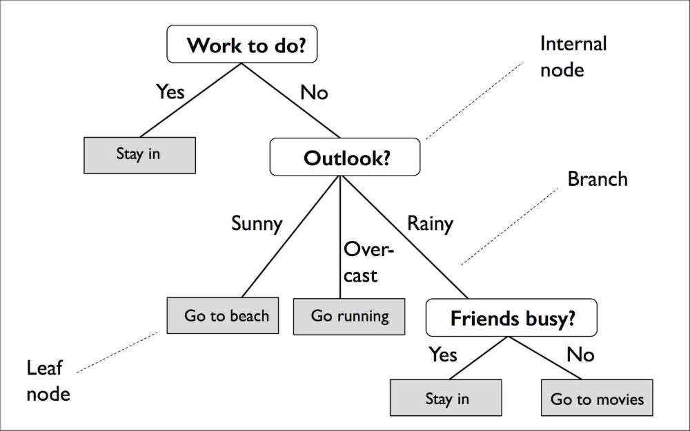
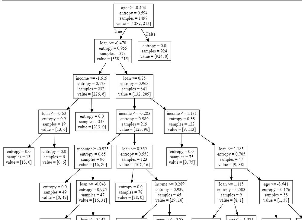
Decision Trees are a non-parametric supervised learning method used for both classification and regression tasks. The goal is to create a model that predicts the value of a target variable by learning simple decision rules derived from the data features.

The decision rules are generally in form of if-then-else statements. The deeper the tree, the more complex the rules and fitter the model.

A decision tree gives output in a tree-like graph with nodes. Take this graph as an example, beautifully explained.

Let’s get hands-on experience on how to perform Decision trees.

Decision Tree Classification

#Importing the libraries
import numpy as np
import matplotlib.pyplot as plt
import pandas as pd

#Importing the dataset
dataset = pd.read_csv('credit_data.csv', sep=",")

#drop the missing values
dataset = dataset.dropna()

X = dataset.iloc[:,1:4].values
y = dataset.iloc[:, 4].values

#--------------------------------------------------

#Splitting the dataset into the Training set and Test set
from sklearn.model_selection import train_test_split
X_train, X_test, y_train, y_test = train_test_split(X, y, test_size = 0.25, random_state = 0)

#fearure scaling/Normalization
from sklearn.preprocessing import StandardScaler
sc = StandardScaler()
X_train = sc.fit_transform(X_train)
X_test = sc.transform(X_test)

Up to this part, we have do the basic pre-processing tasks import data, define X and y, split the data into train and test sets, and last normalization that is scaling to narrow it down the magnitude of the spread of the data points.

Now what we will do here is, We will fit our model in Naïve Bayes as well as Decision trees and will compare which one performs better in classification.

# Fitting Naive Bayes to the Training set
from sklearn.naive_bayes import GaussianNB
NB_model = GaussianNB()
NB_model.fit(X_train, y_train)

# Predicting the Test set results
y_pred2 = NB_model.predict(X_test)

#evaluation Metrics
from sklearn import metrics
print('Accuracy Score:', metrics.accuracy_score(y_test, y_pred2))
print('Balanced Accuracy Score:', metrics.balanced_accuracy_score(y_test, y_pred2))
print('Average Precision:',metrics.average_precision_score(y_test, y_pred2))

#Making the Confusion Matrix
from sklearn.metrics import confusion_matrix
cm2 = confusion_matrix(y_test, y_pred2)

#Fitting Decision Tree Classification to the Training set
from sklearn.tree import DecisionTreeClassifier
dt_model = DecisionTreeClassifier(criterion = 'entropy', random_state = 0)
dt_model.fit(X_train, y_train)

#Predicting the Test set results
y_pred = dt_model.predict(X_test)

#Making the Confusion Matrix
from sklearn.metrics import confusion_matrix
cm = confusion_matrix(y_test, y_pred)

#evaluation Metrics
from sklearn import metrics
print('Accuracy Score:', metrics.accuracy_score(y_test, y_pred))
print('Balanced Accuracy Score:', metrics.balanced_accuracy_score(y_test, y_pred))
print('Average Precision:',metrics.average_precision_score(y_test, y_pred))

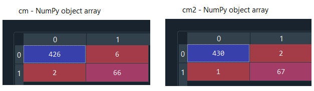
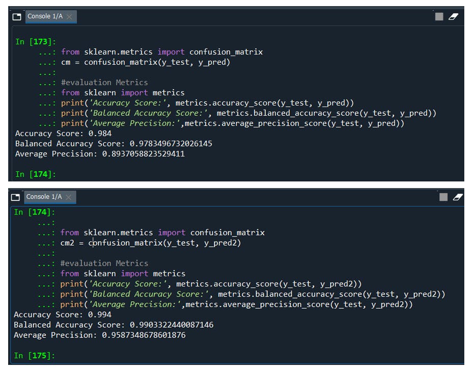
So what we got

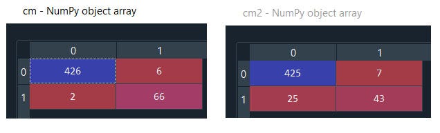
Confusion Matrix, Naive Bayes, Decision Trees — Confusion Matrix | Left| Decision Tree, Right | Naive Bayes

The confusion matrix of Decision Tree is performing better in identifying True Positive and True Negative than Naïve Bayes.

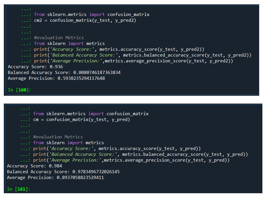
Accuracy Score of Decision Trees Vs Naive Bayes — cm2 ~ Decision Tree | cm ~ Naive Bayes

The accuracy score of our Decision Tree model is better than Naïve Bayes

Hence Decision Tree performs better than Naïve Bayes.

Finally, with the model, we can predict any new input.

#if income, age, loan = 66952.7,28,8770.1
import numpy as np 
# Create a numpy array 
new_data = np.array([66952.7,28,8770.1]) 
new_data.dtype
new_data.shape
#We need to reshape to match the dimensions
new_data = new_data.reshape(-1,3)
new_data.shape
#------------------------------------
from sklearn.preprocessing import StandardScaler
sc= StandardScaler()
#scale the data
new_data = sc.fit_transform(new_data)
#We might see the scaled data as 0, 0, 0 but its not its 0.000000e+ and can be view by changing the format
#else inverse transform will give back the original value
inversed = sc.inverse_transform(new_data)
print(inversed)
#-------------------------------------
dt_model.predict(new_data)

#if we wish to enter manually
dt_model.predict([[66952.7,28,8770.1]])

We have an output of array([0], dtype=int64) that is ‘0’ class. Done… we have classified if income, age, loan = 66952.7, 28, 8770.1 seems will to be a non-defaulter (class=’0') with Decision Tree model.

Its time to visualize the decision tree,

#import export_graphviz
 from sklearn.tree import export_graphviz# export the decision tree to a tree.dot file
#for visualizing the plot easily anywhere
 export_graphviz(dt_model, out_file ='e:/tree.dot',feature_names =['Pressure'])

The tree is finally exported and we can visualize using http://www.webgraphviz.com/ by copying the data from the ‘tree.dot’ file.

Decision Tree Classification with http://www.webgraphviz.com/

Putting all these together the who code looks something like this.

#Decision Tree Classification 
#Importing the libraries
import numpy as np
import matplotlib.pyplot as plt
import pandas as pd

#Importing the dataset
dataset = pd.read_csv('credit_data.csv', sep=",")

#drop the missing values
dataset = dataset.dropna()

X = dataset.iloc[:,1:4].values
y = dataset.iloc[:, 4].values

#----------------------------------------------------
#Splitting the dataset into the Training set and Test set
from sklearn.model_selection import train_test_split
X_train, X_test, y_train, y_test = train_test_split(X, y, test_size = 0.25, random_state = 0)

#fearure scaling/Normalization
from sklearn.preprocessing import StandardScaler
sc = StandardScaler()
X_train = sc.fit_transform(X_train)
X_test = sc.transform(X_test)

#---------------------------------------------------------

#Fitting Naive Bayes to the Training set
from sklearn.naive_bayes import GaussianNB
NB_model = GaussianNB()
NB_model.fit(X_train, y_train)

#Predicting the Test set results
y_pred2 = NB_model.predict(X_test)

#Making the Confusion Matrix
from sklearn.metrics import confusion_matrix
cm2 = confusion_matrix(y_test, y_pred2)

#evaluation Metrics 
from sklearn import metrics
print('Accuracy Score:', metrics.accuracy_score(y_test, y_pred2))  
print('Balanced Accuracy Score:', metrics.balanced_accuracy_score(y_test, y_pred2)) 
print('Average Precision:',metrics.average_precision_score(y_test, y_pred2))

#if income, age, loan = 
NB_model.predict([[66952.7,18,8770.1]])

NB_model.predict([[0.382027,-0.979416,1.45499]])

#-----------------------------------------------------

# Fitting Decision Tree Classification to the Training set
from sklearn.tree import DecisionTreeClassifier
dt_model = DecisionTreeClassifier(criterion = 'entropy', random_state = 0)
dt_model.fit(X_train, y_train)

# Predicting the Test set results
y_pred = dt_model.predict(X_test)

# Making the Confusion Matrix 
from sklearn.metrics import confusion_matrix
cm = confusion_matrix(y_test, y_pred)

#evaluation Metrics 
from sklearn import metrics
print('Accuracy Score:', metrics.accuracy_score(y_test, y_pred))  
print('Balanced Accuracy Score:', metrics.balanced_accuracy_score(y_test, y_pred)) 
print('Average Precision:',metrics.average_precision_score(y_test, y_pred))

from sklearn.tree import export_graphviz  
  # export the decision tree to a tree.dot file 
# for visualizing the plot easily anywhere 
export_graphviz(dt_model, out_file ='e:/tree.dot', 
               feature_names =['income','age','loan'])

"""
The tree is finally exported and we can visualized using  
http://www.webgraphviz.com/ by copying the data from the ‘tree.dot’ file."""

#if income, age, loan = 66952.7,28,8770.1
import numpy as np 
# Create a numpy array 
new_data = np.array([66952.7,28,8770.1]) 
new_data.dtype
new_data.shape
#We need to reshape to match the dimensions
new_data = new_data.reshape(-1,3)
new_data.shape
#------------------------------------
from sklearn.preprocessing import StandardScaler
sc= StandardScaler()
#scale the data
new_data = sc.fit_transform(new_data)
#We might see the scaled data as 0, 0, 0 but its not its 0.000000e+ and can be view by changing the format
#else inverse transform will give back the original value
inversed = sc.inverse_transform(new_data)
print(inversed)
#-------------------------------------
dt_model.predict(new_data)

#if we wish to enter manually
dt_model.predict([[66952.7,28,8770.1]])

Here we are, we have finished how to apply decision trees for non-linear data

NEXT RANDOM FOREST

Introducing Random Forest for Classification

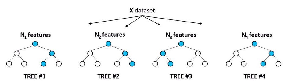
What is a random forest?

Random Forest is the upgrade version of decision trees. The name itself refers it consists of a large number of individual decision trees that operate as an ensemble. Thus we are combining the predictive power of several decision trees to give more accuracy.

Let’s get started with the help of an example

#Random Forest Classification

# Importing the libraries
import numpy as np
import matplotlib.pyplot as plt
import pandas as pd

# Importing the dataset
dataset = pd.read_csv('credit_data.csv', sep=",")

#drop the missing values
dataset = dataset.dropna()

X = dataset.iloc[:,1:4].values
y = dataset.iloc[:, 4].values

#---------------------------------------------------
# Splitting the dataset into the Training set and Test set
from sklearn.model_selection import train_test_split
X_train, X_test, y_train, y_test = train_test_split(X, y, test_size = 0.25, random_state = 0)

#fearure scaling/Normalization
from sklearn.preprocessing import StandardScaler
sc = StandardScaler()
X_train = sc.fit_transform(X_train)
X_test = sc.transform(X_test)

Till here it’s the same basic data pre-processing step from loading the data, defining X & Y, splitting the data into train, and test to data normalization/scaling to reduce the magnitude of the spread of data points.

Now we will fit the random forest into the dataset. Also, we will do for decision tree so that later we can compare the performance.

#Fitting Decision Tree Classification to the Training set
from sklearn.tree import DecisionTreeClassifier
dt_model = DecisionTreeClassifier(criterion = 'entropy', random_state = 0)
dt_model.fit(X_train, y_train)

#Predicting the Test set results
y_pred = dt_model.predict(X_test)

#Making the Confusion Matrix 
from sklearn.metrics import confusion_matrix
cm = confusion_matrix(y_test, y_pred)
 
#evaluation Metrics 
from sklearn import metrics
print('Accuracy Score:', metrics.accuracy_score(y_test, y_pred))  
print('Balanced Accuracy Score:', metrics.balanced_accuracy_score(y_test, y_pred)) 
print('Average Precision:',metrics.average_precision_score(y_test, y_pred))

#------------------------------------------------------------

#Fitting Random Forest Classification to the Training set
from sklearn.ensemble import RandomForestClassifier
rf_model = RandomForestClassifier(n_estimators = 500, criterion = 'entropy', random_state = 0)
rf_model.fit(X_train, y_train)

#Predicting the Test set results
y_pred2 = rf_model.predict(X_test)

#Making the Confusion Matrix
from sklearn.metrics import confusion_matrix
cm2 = confusion_matrix(y_test, y_pred2)

#evaluation Metrics 
from sklearn import metrics
print('Accuracy Score:', metrics.accuracy_score(y_test, y_pred2))  
print('Balanced Accuracy Score:', metrics.balanced_accuracy_score(y_test, y_pred2)) 
print('Average Precision:',metrics.average_precision_score(y_test, y_pred2))

Confusion Matrix: Left | cm | Decision Tree, Right | cm2 | Random Forest

Accuracy Score: Decision Trees 98% | Random Forest 99%

Wwowwww ! we have a 99% model accuracy score. How about yours?

let me know if u need anything or even the data set as this blog doesn’t support file hosting. Ping me @ inbox

Congratulations! we have completed all,,,, yes I would say all the kinds of classification techniques available till today.

It's a long blog, I tried to keep it as short as possible. I hope you have enjoyed it.

I will also be making another version in R. Have a good day. Keep in touch!

Search This Blog

Welcome to #bobrupakroy